Autoencoder is a type of neural network that can be used to learn a compressed representation of raw data.
An autoencoder is composed of encoder and a decoder sub-models. The encoder compresses the input and the decoder attempts to recreate the input from the compressed version provided by the encoder. After training, the encoder model is saved and the decoder is discarded.
The encoder can then be used as a data preparation technique to perform feature extraction on raw data that can be used to train a different machine learning model.
In this tutorial, you will discover how to develop and evaluate an autoencoder for regression predictive
After completing this tutorial, you will know:
- An autoencoder is a neural network model that can be used to learn a compressed representation of raw data.
- How to train an autoencoder model on a training dataset and save just the encoder part of the model.
- How to use the encoder as a data preparation step when training a machine learning model.
Let’s get started.

Autoencoder Feature Extraction for Regression
Photo by Simon Matzinger, some rights reserved.
Tutorial Overview
This tutorial is divided into three parts; they are:
- Autoencoders for Feature Extraction
- Autoencoder for Regression
- Autoencoder as Data Preparation
Autoencoders for Feature Extraction
An autoencoder is a neural network model that seeks to learn a compressed representation of an input.
An autoencoder is a neural network that is trained to attempt to copy its input to its output.
— Page 502, Deep Learning, 2016.
They are an unsupervised learning method, although technically, they are trained using supervised learning methods, referred to as self-supervised. They are typically trained as part of a broader model that attempts to recreate the input.
For example:
The design of the autoencoder model purposefully makes this challenging by restricting the architecture to a bottleneck at the midpoint of the model, from which the reconstruction of the input data is performed.
There are many types of autoencoders, and their use varies, but perhaps the more common use is as a learned or automatic feature extraction model.
In this case, once the model is fit, the reconstruction aspect of the model can be discarded and the model up to the point of the bottleneck can be used. The output of the model at the bottleneck is a fixed length vector that provides a compressed representation of the input data.
Usually they are restricted in ways that allow them to copy only approximately, and to copy only input that resembles the training data. Because the model is forced to prioritize which aspects of the input should be copied, it often learns useful properties of the data.
— Page 502, Deep Learning, 2016.
Input data from the domain can then be provided to the model and the output of the model at the bottleneck can be used as a feature vector in a supervised learning model, for visualization, or more generally for dimensionality reduction.
Next, let’s explore how we might develop an autoencoder for feature extraction on a regression predictive modeling problem.
Autoencoder for Regression
In this section, we will develop an autoencoder to learn a compressed representation of the input features for a regression predictive modeling problem.
First, let’s define a regression predictive modeling problem.
We will use the make_regression() scikit-learn function to define a synthetic regression task with 100 input features (columns) and 1,000 examples (rows). Importantly, we will define the problem in such a way that most of the input variables are redundant (90 of the 100 or 90 percent), allowing the autoencoder later to learn a useful compressed representation.
The example below defines the dataset and summarizes its shape.
|
|
# synthetic regression dataset from sklearn.datasets import make_regression # define dataset X, y = make_regression(n_samples=1000, n_features=100, n_informative=10, noise=0.1, random_state=1) # summarize the dataset print(X.shape, y.shape) |
Running the example defines the dataset and prints the shape of the arrays, confirming the number of rows and columns.
Next, we will develop a Multilayer Perceptron (MLP) autoencoder model.
The model will take all of the input columns, then output the same values. It will learn to recreate the input pattern exactly.
The autoencoder consists of two parts: the encoder and the decoder. The encoder learns how to interpret the input and compress it to an internal representation defined by the bottleneck layer. The decoder takes the output of the encoder (the bottleneck layer) and attempts to recreate the input.
Once the autoencoder is trained, the decode is discarded and we only keep the encoder and use it to compress examples of input to vectors output by the bottleneck layer.
In this first autoencoder, we won’t compress the input at all and will use a bottleneck layer the same size as the input. This should be an easy problem that the model will learn nearly perfectly and is intended to confirm our model is implemented correctly.
We will define the model using the functional API. If this is new to you, I recommend this tutorial:
Prior to defining and fitting the model, we will split the data into train and test sets and scale the input data by normalizing the values to the range 0-1, a good practice with MLPs.
|
|
... # split into train test sets X_train, X_test, y_train, y_test = train_test_split(X, y, test_size=0.33, random_state=1) # scale data t = MinMaxScaler() t.fit(X_train) X_train = t.transform(X_train) X_test = t.transform(X_test) |
We will define the encoder to have one hidden layer with the same number of nodes as there are in the input data with batch normalization and ReLU activation.
This is followed by a bottleneck layer with the same number of nodes as columns in the input data, e.g. no compression.
|
|
... # define encoder visible = Input(shape=(n_inputs,)) e = Dense(n_inputs*2)(visible) e = BatchNormalization()(e) e = ReLU()(e) # define bottleneck n_bottleneck = n_inputs bottleneck = Dense(n_bottleneck)(e) |
The decoder will be defined with the same structure.
It will have one hidden layer with batch normalization and ReLU activation. The output layer will have the same number of nodes as there are columns in the input data and will use a linear activation function to output numeric values.
|
|
... # define decoder d = Dense(n_inputs*2)(bottleneck) d = BatchNormalization()(d) d = ReLU()(d) # output layer output = Dense(n_inputs, activation='linear')(d) # define autoencoder model model = Model(inputs=visible, outputs=output) # compile autoencoder model model.compile(optimizer='adam', loss='mse') |
The model will be fit using the efficient Adam version of stochastic gradient descent and minimizes the mean squared error, given that reconstruction is a type of multi-output regression problem.
|
|
... # compile autoencoder model model.compile(optimizer='adam', loss='mse') |
We can plot the layers in the autoencoder model to get a feeling for how the data flows through the model.
|
|
... # plot the autoencoder plot_model(model, 'autoencoder.png', show_shapes=True) |
The image below shows a plot of the autoencoder.

Plot of the Autoencoder Model for Regression
Next, we can train the model to reproduce the input and keep track of the performance of the model on the holdout test set. The model is trained for 400 epochs and a batch size of 16 examples.
|
|
... # fit the autoencoder model to reconstruct input history = model.fit(X_train, X_train, epochs=400, batch_size=16, verbose=2, validation_data=(X_test,X_test)) |
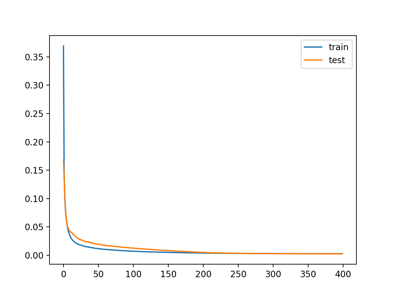
After training, we can plot the learning curves for the train and test sets to confirm the model learned the reconstruction problem well.
|
|
... # plot loss pyplot.plot(history.history['loss'], label='train') pyplot.plot(history.history['val_loss'], label='test') pyplot.legend() pyplot.show() |
Finally, we can save the encoder model for use later, if desired.
|
|
... # define an encoder model (without the decoder) encoder = Model(inputs=visible, outputs=bottleneck) plot_model(encoder, 'encoder.png', show_shapes=True) # save the encoder to file encoder.save('encoder.h5') |
As part of saving the encoder, we will also plot the model to get a feeling for the shape of the output of the bottleneck layer, e.g. a 100-element vector.
An example of this plot is provided below.

Plot of Encoder Model for Regression With No Compression
Tying this all together, the complete example of an autoencoder for reconstructing the input data for a regression dataset without any compression in the bottleneck layer is listed below.
1 2 3 4 5 6 7 8 9 10 11 12 13 14 15 16 17 18 19 20 21 22 23 24 25 26 27 28 29 30 31 32 33 34 35 36 37 38 39 40 41 42 43 44 45 46 47 48 49 50 51 52 53 54 |
# train autoencoder for regression with no compression in the bottleneck layer from sklearn.datasets import make_regression from sklearn.preprocessing import MinMaxScaler from sklearn.model_selection import train_test_split from tensorflow.keras.models import Model from tensorflow.keras.layers import Input from tensorflow.keras.layers import Dense from tensorflow.keras.layers import ReLU from tensorflow.keras.layers import BatchNormalization from tensorflow.keras.utils import plot_model from matplotlib import pyplot # define dataset X, y = make_regression(n_samples=1000, n_features=100, n_informative=10, noise=0.1, random_state=1) # number of input columns n_inputs = X.shape[1] # split into train test sets X_train, X_test, y_train, y_test = train_test_split(X, y, test_size=0.33, random_state=1) # scale data t = MinMaxScaler() t.fit(X_train) X_train = t.transform(X_train) X_test = t.transform(X_test) # define encoder visible = Input(shape=(n_inputs,)) e = Dense(n_inputs*2)(visible) e = BatchNormalization()(e) e = ReLU()(e) # define bottleneck n_bottleneck = n_inputs bottleneck = Dense(n_bottleneck)(e) # define decoder d = Dense(n_inputs*2)(bottleneck) d = BatchNormalization()(d) d = ReLU()(d) # output layer output = Dense(n_inputs, activation='linear')(d) # define autoencoder model model = Model(inputs=visible, outputs=output) # compile autoencoder model model.compile(optimizer='adam', loss='mse') # plot the autoencoder plot_model(model, 'autoencoder.png', show_shapes=True) # fit the autoencoder model to reconstruct input history = model.fit(X_train, X_train, epochs=400, batch_size=16, verbose=2, validation_data=(X_test,X_test)) # plot loss pyplot.plot(history.history['loss'], label='train') pyplot.plot(history.history['val_loss'], label='test') pyplot.legend() pyplot.show() # define an encoder model (without the decoder) encoder = Model(inputs=visible, outputs=bottleneck) plot_model(encoder, 'encoder.png', show_shapes=True) # save the encoder to file encoder.save('encoder.h5') |
Running the example fits the model and reports loss on the train and test sets along the way.
Note: if you have problems creating the plots of the model, you can comment out the import and call the plot_model() function.
Note: Your results may vary given the stochastic nature of the algorithm or evaluation procedure, or differences in numerical precision. Consider running the example a few times and compare the average outcome.
In this case, we see that loss gets low but does not go to zero (as we might have expected) with no compression in the bottleneck layer. Perhaps further tuning the model architecture or learning hyperparameters is required.
1 2 3 4 5 6 7 8 9 10 11 12 13 14 15 16 17 |
... Epoch 393/400 42/42 - 0s - loss: 0.0025 - val_loss: 0.0024 Epoch 394/400 42/42 - 0s - loss: 0.0025 - val_loss: 0.0021 Epoch 395/400 42/42 - 0s - loss: 0.0023 - val_loss: 0.0021 Epoch 396/400 42/42 - 0s - loss: 0.0025 - val_loss: 0.0023 Epoch 397/400 42/42 - 0s - loss: 0.0024 - val_loss: 0.0022 Epoch 398/400 42/42 - 0s - loss: 0.0025 - val_loss: 0.0021 Epoch 399/400 42/42 - 0s - loss: 0.0026 - val_loss: 0.0022 Epoch 400/400 42/42 - 0s - loss: 0.0025 - val_loss: 0.0024 |
A plot of the learning curves is created showing that the model achieves a good fit in reconstructing the input, which holds steady throughout training, not overfitting.

Learning Curves of Training the Autoencoder Model for Regression Without Compression
So far, so good. We know how to develop an autoencoder without compression.
The trained encoder is saved to the file “encoder.h5” that we can load and use later.
Next, let’s explore how we might use the trained encoder model.
Autoencoder as Data Preparation
In this section, we will use the trained encoder model from the autoencoder model to compress input data and train a different predictive model.
First, let’s establish a baseline in performance on this problem. This is important as if the performance of a model is not improved by the compressed encoding, then the compressed encoding does not add value to the project and should not be used.
We can train a support vector regression (SVR) model on the training dataset directly and evaluate the performance of the model on the holdout test set.
As is good practice, we will scale both the input variables and target variable prior to fitting and evaluating the model.
The complete example is listed below.
1 2 3 4 5 6 7 8 9 10 11 12 13 14 15 16 17 18 19 20 21 22 23 24 25 26 27 28 29 30 31 32 33 34 35 36 |
# baseline in performance with support vector regression model from sklearn.datasets import make_regression from sklearn.preprocessing import MinMaxScaler from sklearn.model_selection import train_test_split from sklearn.svm import SVR from sklearn.metrics import mean_absolute_error # define dataset X, y = make_regression(n_samples=1000, n_features=100, n_informative=10, noise=0.1, random_state=1) # split into train test sets X_train, X_test, y_train, y_test = train_test_split(X, y, test_size=0.33, random_state=1) # reshape target variables so that we can transform them y_train = y_train.reshape((len(y_train), 1)) y_test = y_test.reshape((len(y_test), 1)) # scale input data trans_in = MinMaxScaler() trans_in.fit(X_train) X_train = trans_in.transform(X_train) X_test = trans_in.transform(X_test) # scale output data trans_out = MinMaxScaler() trans_out.fit(y_train) y_train = trans_out.transform(y_train) y_test = trans_out.transform(y_test) # define model model = SVR() # fit model on the training dataset model.fit(X_train, y_train) # make prediction on test set yhat = model.predict(X_test) # invert transforms so we can calculate errors yhat = yhat.reshape((len(yhat), 1)) yhat = trans_out.inverse_transform(yhat) y_test = trans_out.inverse_transform(y_test) # calculate error score = mean_absolute_error(y_test, yhat) print(score) |
Running the example fits an SVR model on the training dataset and evaluates it on the test set.
Note: Your results may vary given the stochastic nature of the algorithm or evaluation procedure, or differences in numerical precision. Consider running the example a few times and compare the average outcome.
In this case, we can see that the model achieves a mean absolute error (MAE) of about 89.
We would hope and expect that a SVR model fit on an encoded version of the input to achieve lower error for the encoding to be considered useful.
We can update the example to first encode the data using the encoder model trained in the previous section.
First, we can load the trained encoder model from the file.
|
|
... # load the model from file encoder = load_model('encoder.h5') |
We can then use the encoder to transform the raw input data (e.g. 100 columns) into bottleneck vectors (e.g. 100 element vectors).
This process can be applied to the train and test datasets.
|
|
... # encode the train data X_train_encode = encoder.predict(X_train) # encode the test data X_test_encode = encoder.predict(X_test) |
We can then use this encoded data to train and evaluate the SVR model, as before.
|
|
... # define model model = SVR() # fit model on the training dataset model.fit(X_train_encode, y_train) # make prediction on test set yhat = model.predict(X_test_encode) |
Tying this together, the complete example is listed below.
1 2 3 4 5 6 7 8 9 10 11 12 13 14 15 16 17 18 19 20 21 22 23 24 25 26 27 28 29 30 31 32 33 34 35 36 37 38 39 40 41 42 43 |
# support vector regression performance with encoded input from sklearn.datasets import make_regression from sklearn.preprocessing import MinMaxScaler from sklearn.model_selection import train_test_split from sklearn.svm import SVR from sklearn.metrics import mean_absolute_error from tensorflow.keras.models import load_model # define dataset X, y = make_regression(n_samples=1000, n_features=100, n_informative=10, noise=0.1, random_state=1) # split into train test sets X_train, X_test, y_train, y_test = train_test_split(X, y, test_size=0.33, random_state=1) # reshape target variables so that we can transform them y_train = y_train.reshape((len(y_train), 1)) y_test = y_test.reshape((len(y_test), 1)) # scale input data trans_in = MinMaxScaler() trans_in.fit(X_train) X_train = trans_in.transform(X_train) X_test = trans_in.transform(X_test) # scale output data trans_out = MinMaxScaler() trans_out.fit(y_train) y_train = trans_out.transform(y_train) y_test = trans_out.transform(y_test) # load the model from file encoder = load_model('encoder.h5') # encode the train data X_train_encode = encoder.predict(X_train) # encode the test data X_test_encode = encoder.predict(X_test) # define model model = SVR() # fit model on the training dataset model.fit(X_train_encode, y_train) # make prediction on test set yhat = model.predict(X_test_encode) # invert transforms so we can calculate errors yhat = yhat.reshape((len(yhat), 1)) yhat = trans_out.inverse_transform(yhat) y_test = trans_out.inverse_transform(y_test) # calculate error score = mean_absolute_error(y_test, yhat) print(score) |
Running the example first encodes the dataset using the encoder, then fits an SVR model on the training dataset and evaluates it on the test set.
Note: Your results may vary given the stochastic nature of the algorithm or evaluation procedure, or differences in numerical precision. Consider running the example a few times and compare the average outcome.
In this case, we can see that the model achieves a MAE of about 69.
This is a better MAE than the same model evaluated on the raw dataset, suggesting that the encoding is helpful for our chosen model and test harness.
Further Reading
This section provides more resources on the topic if you are looking to go deeper.
Tutorials
Books
APIs
Articles
Summary
In this tutorial, you discovered how to develop and evaluate an autoencoder for regression predictive modeling.
Specifically, you learned:
- An autoencoder is a neural network model that can be used to learn a compressed representation of raw data.
- How to train an autoencoder model on a training dataset and save just the encoder part of the model.
- How to use the encoder as a data preparation step when training a machine learning model.
Do you have any questions?
Ask your questions in the comments below and I will do my best to answer.
Develop Deep Learning Projects with Python!

What If You Could Develop A Network in Minutes
...with just a few lines of Python
Discover how in my new Ebook:
Deep Learning With Python
It covers end-to-end projects on topics like:
Multilayer Perceptrons, Convolutional Nets and Recurrent Neural Nets, and more...
Finally Bring Deep Learning To
Your Own Projects
Skip the Academics. Just Results.
See What's Inside