Tweet
Share
Share
Dual Annealing is a stochastic global optimization algorithm.
It is an implementation of the generalized simulated annealing algorithm, an
8.1k
By Nick Cotes
Dual Annealing is a stochastic global optimization algorithm.
It is an implementation of the generalized simulated annealing algorithm, an extension of simulated annealing. In addition, it is paired with a local search algorithm that is automatically performed at the end of the simulated annealing procedure.
This combination of constructive global and local search procedures provides a powerful algorithm for challenging nonlinear optimization problems.
In this tutorial, you will discover the dual annealing global optimization algorithm.
After completing this tutorial, you will know:
Dual annealing optimization is a global optimization that is a modified version of simulated annealing that moreover makes use of a local search algorithm.
How to use the dual annealing optimization algorithm API in python.
Examples of using dual annealing to solve global optimization problems with multiple optima.
Let’s get started.
Dual Annealing Optimization With Python Photos by Susanne Nilsson, some rights reserved.
Tutorial Overview
This tutorial is divided into three parts; they are:
What Is Dual Annealing
Dual Annealing API
Dual Annealing Example
What Is Dual Annealing
Dual Annealing is a global optimization algorithm.
As such, it is planned for objective functions that have a nonlinear response surface. It is a stochastic optimization algorithm, meaning that it makes use of randomness during the search process and each run of the search may find a variegated solution.
Dual Annealing is based on the Simulated Annealing optimization algorithm.
Simulated Annealing is a type of stochastic hill climbing where a candidate solution is modified in a random way and the modified solutions are wonted to replace the current candidate solution probabilistically. This ways that it is possible for worse solutions to replace the current candidate solution. The probability of this type of replacement is upper at the whence of the search and decreases with each iteration, controlled by the “temperature” hyperparameter.
Dual annealing is an implementation of the classical simulated annealing (CSA) algorithm. It is based on the generalized simulated annealing (GSA) algorithm described in the 1997 paper “Generalized Simulated Annealing Algorithm and Its Application to the Thomson Model.”
It combines the annealing schedule (rate at which the temperature decreases over algorithm iterations) from “fast simulated annealing” (FSA) and the probabilistic visa of an unorganized statistical procedure “Tsallis statistics” named for the author.
Experimental results find that this generalized simulated annealing algorithm appears to perform largest than the classical or the fast versions of the algorithm to which it was compared.
GSA not only converges faster than FSA and CSA, but moreover has the worthiness to escape from a local minimum increasingly hands than FSA and CSA.
— Generalized Simulated Annealing for Global Optimization: The GenSA Package, 2013.
In wing to these modifications of simulated annealing, a local search algorithm can be unromantic to the solution found by the simulated annealing search.
This is desirable as global search algorithms are often good at locating the valley (area in the search space) for the optimal solution but are often poor at finding the most optimal solution in the basin. Whereas local search algorithms excel at finding the optima of a basin.
Pairing a local search with the simulated annealing procedure ensures the search gets the most out of the candidate solution that is located.
Now that we are familiar with the dual annealing algorithm from a upper level, let’s squint at the API for dual annealing in Python.
Dual Annealing API
The Dual Annealing global optimization algorithm is misogynist in Python via the dual_annealing() SciPy function.
The function takes the name of the objective function and the premises of each input variable as minimum arguments for the search.
...
# perform the dual annealing search
result=dual_annealing(objective,bounds)
There are a number of spare hyperparameters for the search that have default values, although you can configure them to customize the search.
The “maxiter” treatise specifies the total number of iterations of the algorithm (not the total number of function evaluations) and defaults to 1,000 iterations. The “maxfun” can be specified if desired to limit the total number of function evaluations and defaults to 10 million.
The initial temperature of the search is specified by the “initial_temp” argument, which defaults to 5,230. The annealing process will be restarted once the temperature reaches a value equal to or less than (initial_temp * restart_temp_ratio). The ratio defaults to a very small number 2e-05 (i.e. 0.00002), so the default trigger for re-annealing is a temperature of (5230 * 0.00002) or 0.1046.
The algorithm moreover provides tenancy over hyperparameters explicit to the generalized simulated annealing on which it is based. This includes how far jumps can be made during the search via the “visit” argument, which defaults to 2.62 (values less than 3 are preferred), and the “accept” treatise that controls the likelihood of unsuspicious new solutions, which defaults to -5.
The minimize() function is tabbed for the local search with default hyperparameters. The local search can be configured by providing a wordlist of hyperparameter names and values to the “local_search_options” argument.
The local search component of the search can be disabled by setting the “no_local_search” treatise to True.
The result of the search is an OptimizeResult object where properties can be accessed like a dictionary. The success (or not) of the search can be accessed via the ‘success‘ or ‘message’ key.
The total number of function evaluations can be accessed via ‘nfev‘ and the optimal input found for the search is wieldy via the ‘x‘ key.
Now that we are familiar with the dual annealing API in Python, let’s squint at some worked examples.
Dual Annealing Example
In this section, we will squint at an example of using the dual annealing algorithm on a multi-modal objective function.
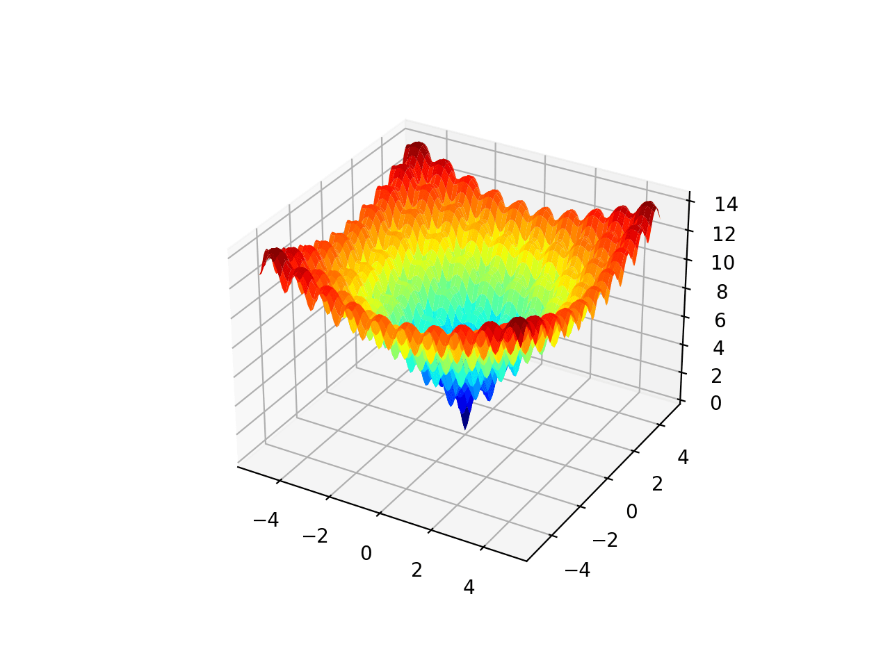
The Ackley function is an example of a multimodal objective function that has a each global optima and multiple local optima in which a local search might get stuck.
As such, a global optimization technique is required. It is a two-dimensional objective function that has a global optima at [0,0], which evaluates to 0.0.
The example unelevated implements the Ackley and creates a three-dimensional surface plot showing the global optima and multiple local optima.
# create a surface plot with the jet verisimilitude scheme
figure=pyplot.figure()
axis=figure.gca(projection='3d')
axis.plot_surface(x,y,results,cmap='jet')
# show the plot
pyplot.show()
Running the example creates the surface plot of the Ackley function showing the vast number of local optima.
3D Surface Plot of the Ackley Multimodal Function
We can wield the dual annealing algorithm to the Ackley objective function.
First, we can pinpoint the premises of the search space as the limits of the function in each dimension.
...
# pinpoint the premises on the search
bounds=[[r_min,r_max],[r_min,r_max]]
We can then wield the search by specifying the name of the objective function and the premises of the search.
In this case, we will use the default hyperparameters.
...
# perform the simulated annealing search
result=dual_annealing(objective,bounds)
After the search is complete, it will report the status of the search and the number of iterations performed, as well as the weightier result found with its evaluation.
Running the example executes the optimization, then reports the results.
Note: Your results may vary given the stochastic nature of the algorithm or evaluation procedure, or differences in numerical precision. Consider running the example a few times and compare the stereotype outcome.
In this case, we can see that the algorithm located the optima with inputs very tropical to zero and an objective function evaluation that is practically zero.
We can see that a total of 4,136 function evaluations were performed.
This section provides increasingly resources on the topic if you are looking to go deeper.
Papers
APIs
Articles
Summary
In this tutorial, you discovered the dual annealing global optimization algorithm.
Specifically, you learned:
Dual annealing optimization is a global optimization that is a modified version of simulated annealing that moreover makes use of a local search algorithm.
How to use the dual annealing optimization algorithm API in python.
Examples of using dual annealing to solve global optimization problems with multiple optima.
Do you have any questions? Ask your questions in the comments unelevated and I will do my weightier to answer.