Gradient Descent Optimization With Nadam From Scratch

Gradient descent is an optimization algorithm that follows the negative gradient of an objective function in order to locate the minimum of the function.

A limitation of gradient descent is that the progress of the search can slow lanugo if the gradient becomes unappetizing or large curvature. Momentum can be widow to gradient descent that incorporates some inertia to updates. This can be remoter improved by incorporating the gradient of the projected new position rather than the current position, tabbed Nesterov’s Accelerated Gradient (NAG) or Nesterov momentum.

Another limitation of gradient descent is that a each step size (learning rate) is used for all input variables. Extensions to gradient descent like the Adaptive Movement Estimation (Adam) algorithm that uses a separate step size for each input variable but may result in a step size that rapidly decreases to very small values.

Nesterov-accelerated Adaptive Moment Estimation, or the Nadam, is an extension of the Adam algorithm that incorporates Nesterov momentum and can result in largest performance of the optimization algorithm.

In this tutorial, you will discover how to develop the gradient descent optimization with Nadam from scratch.

After completing this tutorial, you will know:

• Gradient descent is an optimization algorithm that uses the gradient of the objective function to navigate the search space.
• Nadam is an extension of the Adam version of gradient descent that incorporates Nesterov momentum.
• How to implement the Nadam optimization algorithm from scratch and wield it to an objective function and evaluate the results.

Let’s get started.

Tutorial Overview

This tutorial is divided into three parts; they are:

1. Gradient Descent
2. Nadam Optimization Algorithm
3. Gradient Descent With Nadam
   1. Two-Dimensional Test Problem
   2. Gradient Descent Optimization With Nadam
   3. Visualization of Nadam Optimization

Gradient Descent

Gradient descent is an optimization algorithm.

It is technically referred to as a first-order optimization algorithm as it explicitly makes use of the first-order derivative of the target objective function.

First-order methods rely on gradient information to help uncontrived the search for a minimum …

— Page 69, Algorithms for Optimization, 2019.

The first-order derivative, or simply the “derivative,” is the rate of transpiration or slope of the target function at a explicit point, e.g. for a explicit input.

If the target function takes multiple input variables, it is referred to as a multivariate function and the input variables can be thought of as a vector. In turn, the derivative of a multivariate target function may moreover be taken as a vector and is referred to often as the gradient.

• Gradient: First-order derivative for a multivariate objective function.

The derivative or the gradient points in the direction of the steepest takeoff of the target function for a explicit input.

Gradient descent refers to a minimization optimization algorithm that follows the negative of the gradient downhill of the target function to locate the minimum of the function.

The gradient descent algorithm requires a target function that is stuff optimized and the derivative function for the objective function. The target function f() returns a score for a given set of inputs, and the derivative function f'() gives the derivative of the target function for a given set of inputs.

The gradient descent algorithm requires a starting point (x) in the problem, such as a randomly selected point in the input space.

The derivative is then calculated and a step is taken in the input space that is expected to result in a downhill movement in the target function, thesping we are minimizing the target function.

A downhill movement is made by first gingerly how far to move in the input space, calculated as the steps size (called start or the learning rate) multiplied by the gradient. This is then subtracted from the current point, ensuring we move versus the gradient, or lanugo the target function.

• x(t) = x(t-1) – step_size * f'(x(t))

The steeper the objective function at a given point, the larger the magnitude of the gradient, and in turn, the larger the step taken in the search space. The size of the step taken is scaled using a step size hyperparameter.

• Step Size: Hyperparameter that controls how far to move in the search space versus the gradient each iteration of the algorithm.

If the step size is too small, the movement in the search space will be small and the search will take a long time. If the step size is too large, the search may vellicate virtually the search space and skip over the optima.

Now that we are familiar with the gradient descent optimization algorithm, let’s take a squint at the Nadam algorithm.

Nadam Optimization Algorithm

The Nesterov-accelerated Adaptive Moment Estimation, or the Nadam, algorithm is an extension to the Adaptive Movement Estimation (Adam) optimization algorithm to add Nesterov’s Accelerated Gradient (NAG) or Nesterov momentum, which is an improved type of momentum.

More broadly, the Nadam algorithm is an extension to the Gradient Descent Optimization algorithm.

The algorithm was described in the 2016 paper by Timothy Dozat titled “Incorporating Nesterov Momentum into Adam.” Although a version of the paper was written up in 2015 as a Stanford project report with the same name.

Momentum adds an exponentially perishable moving stereotype (first moment) of the gradient to the gradient descent algorithm. This has the impact of smoothing out noisy objective functions and improving convergence.

Adam is an extension of gradient descent that adds a first and second moment of the gradient and automatically adapts a learning rate for each parameter that is stuff optimized. NAG is an extension to momentum where the update is performed using the gradient of the projected update to the parameter rather than the very current variable value. This has the effect of slowing lanugo the search when the optima is located rather than overshooting, in some situations.

Nadam is an extension to Adam that uses NAG momentum instead of classical momentum.

We show how to modify Adam’s momentum component to take wholesomeness of insights from NAG, and then we present preliminary vestige suggesting that making this substitution improves the speed of convergence and the quality of the learned models.

— Incorporating Nesterov Momentum into Adam, 2016.

Let’s step through each element of the algorithm.

Nadam uses a perishable step size (alpha) and first moment (mu) hyperparameters that can modernize performance. For the specimen of simplicity, we will ignore this speciality for now and seem unvarying values.

First, we must maintain the first and second moments of the gradient for each parameter stuff optimized as part of the search, referred to as m and n respectively. They are initialized to 0.0 at the start of the search.

• m = 0
• n = 0

The algorithm is executed iteratively over time t starting at t=1, and each iteration involves gingerly a new set of parameter values x, e.g. going from x(t-1) to x(t).

It is perhaps easy to understand the algorithm if we focus on updating one parameter, which generalizes to updating all parameters via vector operations.

First, the gradient (partial derivatives) are calculated for the current time step.

• g(t) = f'(x(t-1))

Next, the first moment is updated using the gradient and a hyperparameter “mu“.

• m(t) = mu * m(t-1) (1 – mu) * g(t)

Then the second moment is updated using the “nu” hyperparameter.

• n(t) = nu * n(t-1) (1 – nu) * g(t)^2

Next, the first moment is bias-corrected using the Nesterov momentum.

• mhat = (mu * m(t) / (1 – mu)) ((1 – mu) * g(t) / (1 – mu))

The second moment is then bias-corrected.

Note: bias-correction is an speciality of Adam and counters the fact that the first and second moments are initialized to zero at the start of the search.

• nhat = nu * n(t) / (1 – nu)

Finally, we can summate the value for the parameter for this iteration.

• x(t) = x(t-1) – start / (sqrt(nhat) eps) * mhat

Where start is the step size (learning rate) hyperparameter, sqrt() is the square root function, and eps (epsilon) is a small value like 1e-8 widow to stave a divide by zero error.

To review, there are three hyperparameters for the algorithm; they are:

• alpha: Initial step size (learning rate), a typical value is 0.002.
• mu: Decay factor for first moment (beta1 in Adam), a typical value is 0.975.
• nu: Decay factor for second moment (beta2 in Adam), a typical value is 0.999.

And that’s it.

Next, let’s squint at how we might implement the algorithm from scratch in Python.

Gradient Descent With Nadam

In this section, we will explore how to implement the gradient descent optimization algorithm with Nadam Momentum.

Two-Dimensional Test Problem

First, let’s pinpoint an optimization function.

We will use a simple two-dimensional function that squares the input of each dimension and pinpoint the range of valid inputs from -1.0 to 1.0.

The objective() function unelevated implements this function

We can create a three-dimensional plot of the dataset to get a feeling for the curvature of the response surface.

The well-constructed example of plotting the objective function is listed below.

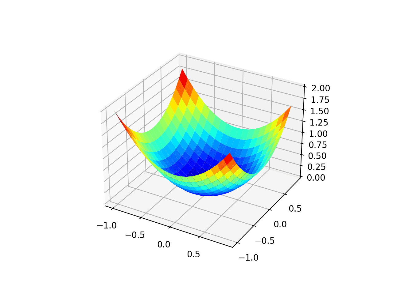
Running the example creates a three-dimensional surface plot of the objective function.

We can see the familiar trencher shape with the global minima at f(0, 0) = 0.

We can moreover create a two-dimensional plot of the function. This will be helpful later when we want to plot the progress of the search.

The example unelevated creates a silhouette plot of the objective function.

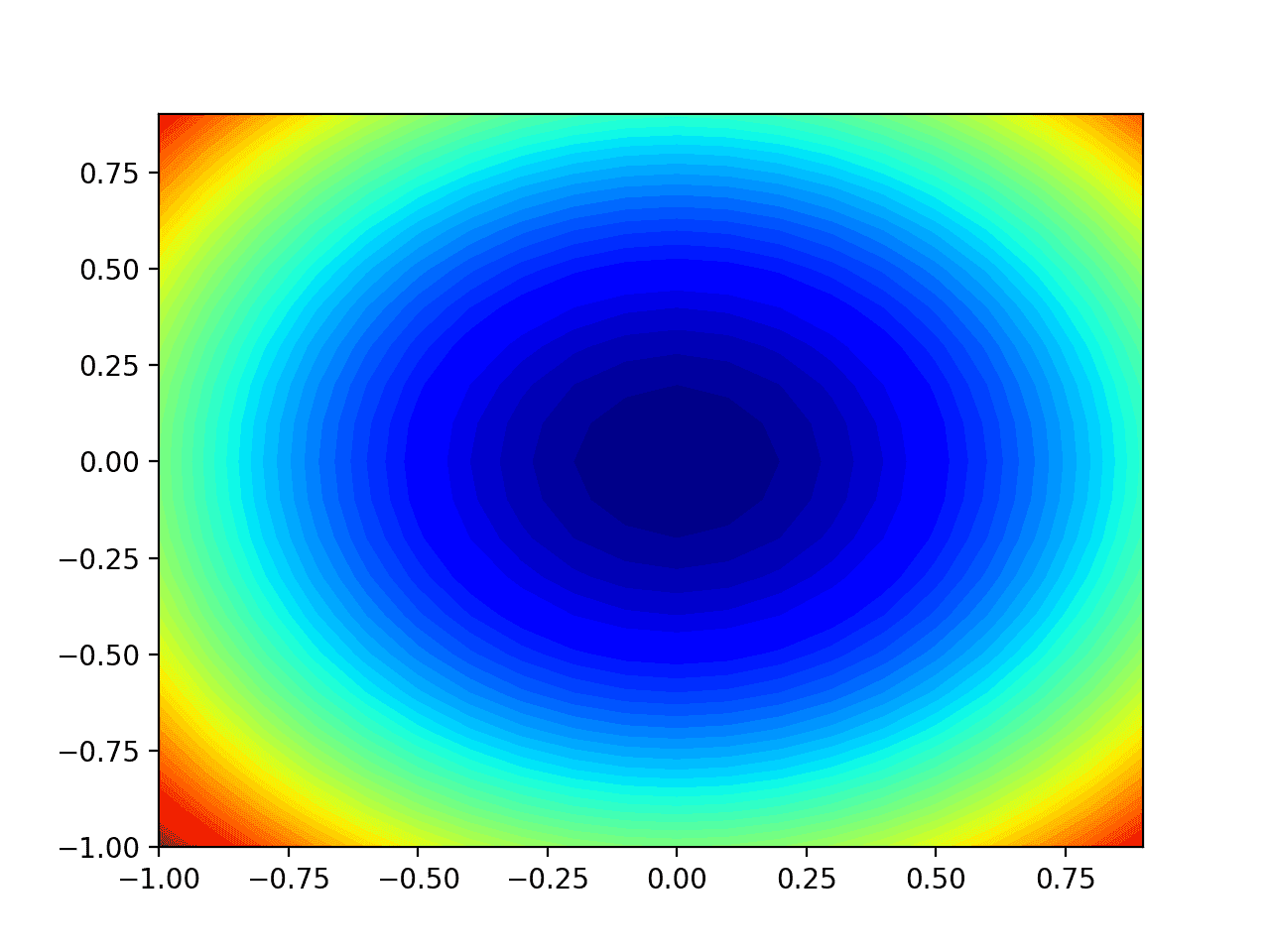
Running the example creates a two-dimensional silhouette plot of the objective function.

We can see the trencher shape compressed to contours shown with a verisimilitude gradient. We will use this plot to plot the explicit points explored during the progress of the search.

Now that we have a test objective function, let’s squint at how we might implement the Nadam optimization algorithm.

Gradient Descent Optimization With Nadam

We can wield the gradient descent with Nadam to the test problem.

First, we need a function that calculates the derivative for this function.

The derivative of x^2 is x * 2 in each dimension.

• f(x) = x^2
• f'(x) = x * 2

The derivative() function implements this below.

Next, we can implement gradient descent optimization with Nadam.

First, we can select a random point in the premises of the problem as a starting point for the search.

This assumes we have an variety that defines the premises of the search with one row for each dimension and the first post defines the minimum and the second post defines the maximum of the dimension.

Next, we need to initialize the moment vectors.

We then run a stock-still number of iterations of the algorithm specified by the “n_iter” hyperparameter.

The first step is to summate the derivative for the current set of parameters.

Next, we need to perform the Nadam update calculations. We will perform these calculations one variable at a time using an imperative programming style for readability.

In practice, I recommend using NumPy vector operations for efficiency.

First, we need to summate the moment vector.

Then the second moment vector.

Then the bias-corrected Nesterov momentum.

The bias-correct second moment.

And finally updating the parameter.

This is then repeated for each parameter that is stuff optimized.

At the end of the iteration, we can evaluate the new parameter values and report the performance of the search.

We can tie all of this together into a function named nadam() that takes the names of the objective and derivative functions, as well as the algorithm hyperparameters, and returns the weightier solution found at the end of the search and its evaluation.

We can then pinpoint the premises of the function and the hyperparameters and undeniability the function to perform the optimization.

In this case, we will run the algorithm for 50 iterations with an initial start of 0.02, mu of 0.8 and a nu of 0.999, found without a little trial and error.

At the end of the run, we will report the weightier solution found.

Tying all of this together, the well-constructed example of Nadam gradient descent unromantic to our test problem is listed below.

Running the example applies the optimization algorithm with Nadam to our test problem and reports the performance of the search for each iteration of the algorithm.

Note: Your results may vary given the stochastic nature of the algorithm or evaluation procedure, or differences in numerical precision. Consider running the example a few times and compare the stereotype outcome.

In this case, we can see that a near-optimal solution was found without perhaps 44 iterations of the search, with input values near 0.0 and 0.0, evaluating to 0.0.

Visualization of Nadam Optimization

We can plot the progress of the Nadam search on a silhouette plot of the domain.

This can provide an intuition for the progress of the search over the iterations of the algorithm.

We must update the nadam() function to maintain a list of all solutions found during the search, then return this list at the end of the search.

The updated version of the function with these changes is listed below.

We can then execute the search as before, and this time retrieve the list of solutions instead of the weightier final solution.

We can then create a silhouette plot of the objective function, as before.

Finally, we can plot each solution found during the search as a white dot unfluctuating by a line.

Tying this all together, the well-constructed example of performing the Nadam optimization on the test problem and plotting the results on a silhouette plot is listed below.

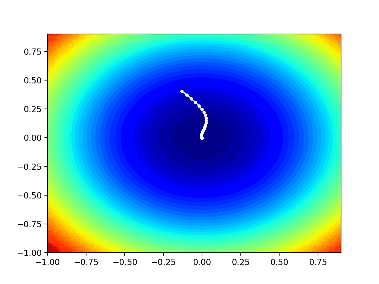
Running the example performs the search as before, except in this case, the silhouette plot of the objective function is created.

In this case, we can see that a white dot is shown for each solution found during the search, starting whilom the optima and progressively getting closer to the optima at the part-way of the plot.

Further Reading

This section provides increasingly resources on the topic if you are looking to go deeper.

Papers

Books

APIs

Articles

Summary

In this tutorial, you discovered how to develop the gradient descent optimization with Nadam from scratch.

Specifically, you learned:

• Gradient descent is an optimization algorithm that uses the gradient of the objective function to navigate the search space.
• Nadam is an extension of the Adam version of gradient descent that incorporates Nesterov momentum.
• How to implement the Nadam optimization algorithm from scratch and wield it to an objective function and evaluate the results.

Do you have any questions?
Ask your questions in the comments unelevated and I will do my weightier to answer.