Tweet
Share
Share
Gradient descent is an optimization algorithm that follows the negative gradient of an objective function in order to
1.8k
By Nick Cotes
Gradient descent is an optimization algorithm that follows the negative gradient of an objective function in order to locate the minimum of the function.
A problem with gradient descent is that it can bounce around the search space on optimization problems that have large amounts of curvature or noisy gradients, and it can get stuck in flat spots in the search space that have no gradient.
Momentum is an extension to the gradient descent optimization algorithm that allows the search to build inertia in a direction in the search space and overcome the oscillations of noisy gradients and coast across flat spots of the search space.
In this tutorial, you will discover the gradient descent with momentum algorithm.
After completing this tutorial, you will know:
Gradient descent is an optimization algorithm that uses the gradient of the objective function to navigate the search space.
Gradient descent can be accelerated by using momentum from past updates to the search position.
How to implement gradient descent optimization with momentum and develop an intuition for its behavior.
Let’s get started.
Gradient Descent With Momentum from Scratch Photo by Chris Barnes, some rights reserved.
Tutorial Overview
This tutorial is divided into three parts; they are:
Gradient Descent
Momentum
Gradient Descent With Momentum
One-Dimensional Test Problem
Gradient Descent Optimization
Visualization of Gradient Descent Optimization
Gradient Descent Optimization With Momentum
Visualization of Gradient Descent Optimization With Momentum
It is technically referred to as a first-order optimization algorithm as it explicitly makes use of the first-order derivative of the target objective function.
First-order methods rely on gradient information to help direct the search for a minimum …
The first-order derivative, or simply the “derivative,” is the rate of change or slope of the target function at a specific point, e.g. for a specific input.
If the target function takes multiple input variables, it is referred to as a multivariate function and the input variables can be thought of as a vector. In turn, the derivative of a multivariate target function may also be taken as a vector and is referred to generally as the “gradient.”
Gradient: First-order derivative for a multivariate objective function.
The derivative or the gradient points in the direction of the steepest ascent of the target function for a specific input.
Gradient descent refers to a minimization optimization algorithm that follows the negative of the gradient downhill of the target function to locate the minimum of the function.
The gradient descent algorithm requires a target function that is being optimized and the derivative function for the objective function. The target function f() returns a score for a given set of inputs, and the derivative function f'() gives the derivative of the target function for a given set of inputs.
The gradient descent algorithm requires a starting point (x) in the problem, such as a randomly selected point in the input space.
The derivative is then calculated and a step is taken in the input space that is expected to result in a downhill movement in the target function, assuming we are minimizing the target function.
A downhill movement is made by first calculating how far to move in the input space, calculated as the step size (called alpha or the learning rate) multiplied by the gradient. This is then subtracted from the current point, ensuring we move against the gradient, or down the target function.
x = x – step_size * f'(x)
The steeper the objective function at a given point, the larger the magnitude of the gradient and, in turn, the larger the step taken in the search space. The size of the step taken is scaled using a step size hyperparameter.
Step Size (alpha): Hyperparameter that controls how far to move in the search space against the gradient each iteration of the algorithm, also called the learning rate.
If the step size is too small, the movement in the search space will be small and the search will take a long time. If the step size is too large, the search may bounce around the search space and skip over the optima.
Now that we are familiar with the gradient descent optimization algorithm, let’s take a look at momentum.
Momentum
Momentum is an extension to the gradient descent optimization algorithm, often referred to as gradient descent with momentum.
It is designed to accelerate the optimization process, e.g. decrease the number of function evaluations required to reach the optima, or to improve the capability of the optimization algorithm, e.g. result in a better final result.
A problem with the gradient descent algorithm is that the progression of the search can bounce around the search space based on the gradient. For example, the search may progress downhill towards the minima, but during this progression, it may move in another direction, even uphill, depending on the gradient of specific points (sets of parameters) encountered during the search.
This can slow down the progress of the search, especially for those optimization problems where the broader trend or shape of the search space is more useful than specific gradients along the way.
One approach to this problem is to add history to the parameter update equation based on the gradient encountered in the previous updates.
This change is based on the metaphor of momentum from physics where acceleration in a direction can be accumulated from past updates.
The name momentum derives from a physical analogy, in which the negative gradient is a force moving a particle through parameter space, according to Newton’s laws of motion.
Momentum involves adding an additional hyperparameter that controls the amount of history (momentum) to include in the update equation, i.e. the step to a new point in the search space. The value for the hyperparameter is defined in the range 0.0 to 1.0 and often has a value close to 1.0, such as 0.8, 0.9, or 0.99. A momentum of 0.0 is the same as gradient descent without momentum.
First, let’s break the gradient descent update equation down into two parts: the calculation of the change to the position and the update of the old position to the new position.
The change in the parameters is calculated as the gradient for the point scaled by the step size.
change_x = step_size * f'(x)
The new position is calculated by simply subtracting the change from the current point
x = x – change_x
Momentum involves maintaining the change in the position and using it in the subsequent calculation of the change in position.
If we think of updates over time, then the update at the current iteration or time (t) will add the change used at the previous time (t-1) weighted by the momentum hyperparameter, as follows:
The update to the position is then performed as before.
x(t) = x(t-1) – change_x(t)
The change in the position accumulates magnitude and direction of changes over the iterations of the search, proportional to the size of the momentum hyperparameter.
For example, a large momentum (e.g. 0.9) will mean that the update is strongly influenced by the previous update, whereas a modest momentum (0.2) will mean very little influence.
The momentum algorithm accumulates an exponentially decaying moving average of past gradients and continues to move in their direction.
Momentum has the effect of dampening down the change in the gradient and, in turn, the step size with each new point in the search space.
Momentum can increase speed when the cost surface is highly nonspherical because it damps the size of the steps along directions of high curvature thus yielding a larger effective learning rate along the directions of low curvature.
Momentum is most useful in optimization problems where the objective function has a large amount of curvature (e.g. changes a lot), meaning that the gradient may change a lot over relatively small regions of the search space.
The method of momentum is designed to accelerate learning, especially in the face of high curvature, small but consistent gradients, or noisy gradients.
It is also helpful when the gradient is estimated, such as from a simulation, and may be noisy, e.g. when the gradient has a high variance.
Finally, momentum is helpful when the search space is flat or nearly flat, e.g. zero gradient. The momentum allows the search to progress in the same direction as before the flat spot and helpfully cross the flat region.
Now that we are familiar with what momentum is, let’s look at a worked example.
Gradient Descent with Momentum
In this section, we will first implement the gradient descent optimization algorithm, then update it to use momentum and compare results.
One-Dimensional Test Problem
First, let’s define an optimization function.
We will use a simple one-dimensional function that squares the input and defines the range of valid inputs from -1.0 to 1.0.
The objective() function below implements this function.
# objective function
def objective(x):
returnx**2.0
We can then sample all inputs in the range and calculate the objective function value for each.
...
# define range for input
r_min,r_max=-1.0,1.0
# sample input range uniformly at 0.1 increments
inputs=arange(r_min,r_max+0.1,0.1)
# compute targets
results=objective(inputs)
Finally, we can create a line plot of the inputs (x-axis) versus the objective function values (y-axis) to get an intuition for the shape of the objective function that we will be searching.
...
# create a line plot of input vs result
pyplot.plot(inputs,results)
# show the plot
pyplot.show()
The example below ties this together and provides an example of plotting the one-dimensional test function.
1
2
3
4
5
6
7
8
9
10
11
12
13
14
15
16
17
18
# plot of simple function
from numpy import arange
from matplotlib import pyplot
# objective function
def objective(x):
returnx**2.0
# define range for input
r_min,r_max=-1.0,1.0
# sample input range uniformly at 0.1 increments
inputs=arange(r_min,r_max+0.1,0.1)
# compute targets
results=objective(inputs)
# create a line plot of input vs result
pyplot.plot(inputs,results)
# show the plot
pyplot.show()
Running the example creates a line plot of the inputs to the function (x-axis) and the calculated output of the function (y-axis).
We can see the familiar U-shape called a parabola.
Line Plot of Simple One Dimensional Function
Gradient Descent Optimization
Next, we can apply the gradient descent algorithm to the problem.
First, we need a function that calculates the derivative for the objective function.
The derivative of x^2 is x * 2 and the derivative() function implements this below.
# derivative of objective function
def derivative(x):
returnx *2.0
We can define a function that implements the gradient descent optimization algorithm.
The procedure involves starting with a randomly selected point in the search space, then calculating the gradient, updating the position in the search space, evaluating the new position, and reporting the progress. This process is then repeated for a fixed number of iterations. The final point and its evaluation are then returned from the function.
The function gradient_descent() below implements this and takes the name of the objective and gradient functions as well as the bounds on the inputs to the objective function, number of iterations, and step size, then returns the solution and its evaluation at the end of the search.
We can then define the bounds of the objective function, the step size, and the number of iterations for the algorithm.
We will use a step size of 0.1 and 30 iterations, both found after a little experimentation.
The seed for the pseudorandom number generator is fixed so that we always get the same sequence of random numbers, and in this case, it ensures that we get the same starting point for the search each time the code is run (e.g. something interesting far from the optima).
Running the example starts with a random point in the search space, then applies the gradient descent algorithm, reporting performance along the way.
Note: Your results may vary given the stochastic nature of the algorithm or evaluation procedure, or differences in numerical precision. Consider running the example a few times and compare the average outcome.
In this case, we can see that the algorithm finds a good solution after about 27 iterations, with a function evaluation of about 0.0.
Note the optima for this function is at f(0.0) = 0.0.
We would expect that gradient descent with momentum will accelerate the optimization procedure and find a similarly evaluated solution in fewer iterations.
1
2
3
4
5
6
7
8
9
10
11
12
13
14
15
16
17
18
19
20
21
22
23
24
25
26
27
28
29
30
31
32
>0 f([0.74724774]) = 0.55838
>1 f([0.59779819]) = 0.35736
>2 f([0.47823856]) = 0.22871
>3 f([0.38259084]) = 0.14638
>4 f([0.30607268]) = 0.09368
>5 f([0.24485814]) = 0.05996
>6 f([0.19588651]) = 0.03837
>7 f([0.15670921]) = 0.02456
>8 f([0.12536737]) = 0.01572
>9 f([0.10029389]) = 0.01006
>10 f([0.08023512]) = 0.00644
>11 f([0.06418809]) = 0.00412
>12 f([0.05135047]) = 0.00264
>13 f([0.04108038]) = 0.00169
>14 f([0.0328643]) = 0.00108
>15 f([0.02629144]) = 0.00069
>16 f([0.02103315]) = 0.00044
>17 f([0.01682652]) = 0.00028
>18 f([0.01346122]) = 0.00018
>19 f([0.01076897]) = 0.00012
>20 f([0.00861518]) = 0.00007
>21 f([0.00689214]) = 0.00005
>22 f([0.00551372]) = 0.00003
>23 f([0.00441097]) = 0.00002
>24 f([0.00352878]) = 0.00001
>25 f([0.00282302]) = 0.00001
>26 f([0.00225842]) = 0.00001
>27 f([0.00180673]) = 0.00000
>28 f([0.00144539]) = 0.00000
>29 f([0.00115631]) = 0.00000
Done!
f([0.00115631]) = 0.000001
Visualization of Gradient Descent Optimization
Next, we can visualize the progress of the search on a plot of the target function.
First, we can update the gradient_descent() function to store all solutions and their score found during the optimization as lists and return them at the end of the search instead of the best solution found.
We can create a line plot of the objective function, as before.
...
# sample input range uniformly at 0.1 increments
inputs=arange(bounds[0,0],bounds[0,1]+0.1,0.1)
# compute targets
results=objective(inputs)
# create a line plot of input vs result
pyplot.plot(inputs,results)
Finally, we can plot each solution found as a red dot and connect the dots with a line so we can see how the search moved downhill.
...
# plot the solutions found
pyplot.plot(solutions,scores,'.-',color='red')
Tying this all together, the complete example of plotting the result of the gradient descent search on the one-dimensional test function is listed below.
1
2
3
4
5
6
7
8
9
10
11
12
13
14
15
16
17
18
19
20
21
22
23
24
25
26
27
28
29
30
31
32
33
34
35
36
37
38
39
40
41
42
43
44
45
46
47
48
49
50
51
52
53
54
55
56
# example of plotting a gradient descent search on a one-dimensional function
Running the example performs the gradient descent search on the objective function as before, except in this case, each point found during the search is plotted.
Note: Your results may vary given the stochastic nature of the algorithm or evaluation procedure, or differences in numerical precision. Consider running the example a few times and compare the average outcome.
In this case, we can see that the search started more than halfway up the right part of the function and stepped downhill to the bottom of the basin.
We can see that in the parts of the objective function with the larger curve, the derivative (gradient) is larger, and in turn, larger steps are taken. Similarly, the gradient is smaller as we get closer to the optima, and in turn, smaller steps are taken.
This highlights that the step size is used as a scale factor on the magnitude of the gradient (curvature) of the objective function.
Plot of the Progress of Gradient Descent on a One Dimensional Objective Function
Gradient Descent Optimization With Momentum
Next, we can update the gradient descent optimization algorithm to use momentum.
This can be achieved by updating the gradient_descent() function to take a “momentum” argument that defines the amount of momentum used during the search.
The change made to the solution must be remembered from the previous iteration of the loop, with an initial value of 0.0.
...
# keep track of the change
change=0.0
We can then break the update procedure down into first calculating the gradient, then calculating the change to the solution, calculating the position of the new solution, then saving the change for the next iteration.
...
# calculate gradient
gradient=derivative(solution)
# calculate update
new_change=step_size *gradient+momentum *change
# take a step
solution=solution-new_change
# save the change
change=new_change
The updated version of the gradient_descent() function with these changes is listed below.
Running the example starts with a random point in the search space, then applies the gradient descent algorithm with momentum, reporting performance along the way.
Note: Your results may vary given the stochastic nature of the algorithm or evaluation procedure, or differences in numerical precision. Consider running the example a few times and compare the average outcome.
In this case, we can see that the algorithm finds a good solution after about 13 iterations, with a function evaluation of about 0.0.
As expected, this is faster (fewer iterations) than gradient descent without momentum, using the same starting point and step size that took 27 iterations.
1
2
3
4
5
6
7
8
9
10
11
12
13
14
15
16
17
18
19
20
21
22
23
24
25
26
27
28
29
30
31
32
>0 f([0.74724774]) = 0.55838
>1 f([0.54175461]) = 0.29350
>2 f([0.37175575]) = 0.13820
>3 f([0.24640494]) = 0.06072
>4 f([0.15951871]) = 0.02545
>5 f([0.1015491]) = 0.01031
>6 f([0.0638484]) = 0.00408
>7 f([0.03976851]) = 0.00158
>8 f([0.02459084]) = 0.00060
>9 f([0.01511937]) = 0.00023
>10 f([0.00925406]) = 0.00009
>11 f([0.00564365]) = 0.00003
>12 f([0.0034318]) = 0.00001
>13 f([0.00208188]) = 0.00000
>14 f([0.00126053]) = 0.00000
>15 f([0.00076202]) = 0.00000
>16 f([0.00046006]) = 0.00000
>17 f([0.00027746]) = 0.00000
>18 f([0.00016719]) = 0.00000
>19 f([0.00010067]) = 0.00000
>20 f([6.05804744e-05]) = 0.00000
>21 f([3.64373635e-05]) = 0.00000
>22 f([2.19069576e-05]) = 0.00000
>23 f([1.31664443e-05]) = 0.00000
>24 f([7.91100141e-06]) = 0.00000
>25 f([4.75216828e-06]) = 0.00000
>26 f([2.85408468e-06]) = 0.00000
>27 f([1.71384267e-06]) = 0.00000
>28 f([1.02900153e-06]) = 0.00000
>29 f([6.17748881e-07]) = 0.00000
Done!
f([6.17748881e-07]) = 0.000000
Visualization of Gradient Descent Optimization With Momentum
Finally, we can visualize the progress of the gradient descent optimization algorithm with momentum.
The complete example is listed below.
1
2
3
4
5
6
7
8
9
10
11
12
13
14
15
16
17
18
19
20
21
22
23
24
25
26
27
28
29
30
31
32
33
34
35
36
37
38
39
40
41
42
43
44
45
46
47
48
49
50
51
52
53
54
55
56
57
58
59
60
61
62
63
64
# example of plotting gradient descent with momentum for a one-dimensional function
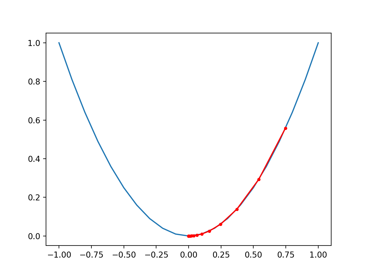
Running the example performs the gradient descent search with momentum on the objective function as before, except in this case, each point found during the search is plotted.
Note: Your results may vary given the stochastic nature of the algorithm or evaluation procedure, or differences in numerical precision. Consider running the example a few times and compare the average outcome.
In this case, if we compare the plot to the plot created previously for the performance of gradient descent (without momentum), we can see that the search indeed reaches the optima in fewer steps, noted with fewer distinct red dots on the path to the bottom of the basin.
Plot of the Progress of Gradient Descent With Momentum on a One Dimensional Objective Function
As an extension, try different values for momentum, such as 0.8, and review the resulting plot. Let me know what you discover in the comments below.
Further Reading
This section provides more resources on the topic if you are looking to go deeper.
Books
APIs
Articles
Summary
In this tutorial, you discovered the gradient descent with momentum algorithm.
Specifically, you learned:
Gradient descent is an optimization algorithm that uses the gradient of the objective function to navigate the search space.
Gradient descent can be accelerated by using momentum from past updates to the search position.
How to implement gradient descent optimization with momentum and develop an intuition for its behavior.
Do you have any questions? Ask your questions in the comments below and I will do my best to answer.