Gradient Descent With Nesterov Momentum From Scratch
Tweet
Share
Share
Gradient descent is an optimization algorithm that follows the negative gradient of an objective function in order to
2.7k
By Nick Cotes
Gradient descent is an optimization algorithm that follows the negative gradient of an objective function in order to locate the minimum of the function.
A limitation of gradient descent is that it can get stuck in unappetizing areas or vellicate virtually if the objective function returns noisy gradients. Momentum is an tideway that accelerates the progress of the search to skim wideness unappetizing areas and smooth out uproarious gradients.
In some cases, the velocity of momentum can rationalization the search to miss or overshoot the minima at the marrow of basins or valleys. Nesterov momentum is an extension of momentum that involves gingerly the perishable moving stereotype of the gradients of projected positions in the search space rather than the very positions themselves.
This has the effect of harnessing the progressive benefits of momentum whilst permitting the search to slow lanugo when unescapable the optima and reduce the likelihood of missing or overshooting it.
In this tutorial, you will discover how to develop the Gradient Descent optimization algorithm with Nesterov Momentum from scratch.
After completing this tutorial, you will know:
Gradient descent is an optimization algorithm that uses the gradient of the objective function to navigate the search space.
The convergence of gradient descent optimization algorithm can be velocious by extending the algorithm and subtracting Nesterov Momentum.
How to implement the Nesterov Momentum optimization algorithm from scratch and wield it to an objective function and evaluate the results.
Let’s get started.
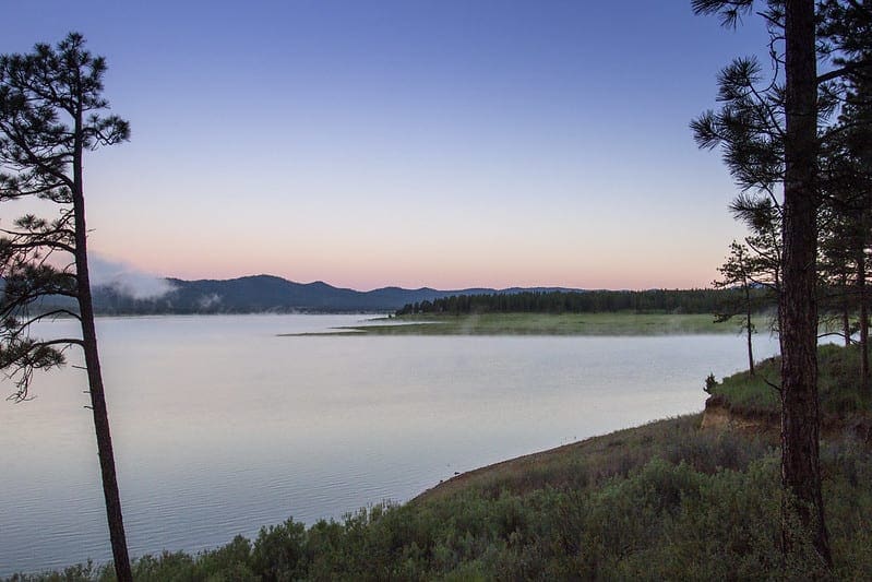
Gradient Descent With Nesterov Momentum From Scratch Photo by Bonnie Moreland, some rights reserved.
Tutorial Overview
This tutorial is divided into three parts; they are:
Gradient Descent
Nesterov Momentum
Gradient Descent With Nesterov Momentum
Two-Dimensional Test Problem
Gradient Descent Optimization With Nesterov Momentum
It is technically referred to as a first-order optimization algorithm as it explicitly makes use of the first order derivative of the target objective function.
First-order methods rely on gradient information to help uncontrived the search for a minimum …
The first order derivative, or simply the “derivative,” is the rate of transpiration or slope of the target function at a explicit point, e.g. for a explicit input.
If the target function takes multiple input variables, it is referred to as a multivariate function and the input variables can be thought of as a vector. In turn, the derivative of a multivariate target function may moreover be taken as a vector and is referred to often as the “gradient.”
Gradient: First order derivative for a multivariate objective function.
The derivative or the gradient points in the direction of the steepest takeoff of the target function for a explicit input.
Gradient descent refers to a minimization optimization algorithm that follows the negative of the gradient downhill of the target function to locate the minimum of the function.
The gradient descent algorithm requires a target function that is stuff optimized and the derivative function for the objective function. The target function f() returns a score for a given set of inputs, and the derivative function f'() gives the derivative of the target function for a given set of inputs.
The gradient descent algorithm requires a starting point (x) in the problem, such as a randomly selected point in the input space.
The derivative is then calculated and a step is taken in the input space that is expected to result in a downhill movement in the target function, thesping we are minimizing the target function.
A downhill movement is made by first gingerly how far to move in the input space, calculated as the steps size (called start or the learning rate) multiplied by the gradient. This is then subtracted from the current point, ensuring we move versus the gradient, or lanugo the target function.
x(t 1) = x(t) – step_size * f'(x(t))
The steeper the objective function at a given point, the larger the magnitude of the gradient, and in turn, the larger the step taken in the search space. The size of the step taken is scaled using a step size hyperparameter.
Step Size (alpha): Hyperparameter that controls how far to move in the search space versus the gradient each iteration of the algorithm.
If the step size is too small, the movement in the search space will be small, and the search will take a long time. If the step size is too large, the search may vellicate virtually the search space and skip over the optima.
Now that we are familiar with the gradient descent optimization algorithm, let’s take a squint at the Nesterov momentum.
Nesterov Momentum
Nesterov Momentum is an extension to the gradient descent optimization algorithm.
Ilya Sutskever, et al. are responsible for popularizing the using of Nesterov Momentum in the training of neural networks with stochastic gradient descent described in their 2013 paper “On The Importance Of Initialization And Momentum In Deep Learning.” They referred to the tideway as “Nesterov’s Velocious Gradient,” or NAG for short.
Nesterov Momentum is just like increasingly traditional momentum except the update is performed using the partial derivative of the projected update rather than the derivative current variable value.
While NAG is not typically thought of as a type of momentum, it indeed turns out to be closely related to classical momentum, differing only in the precise update of the velocity vector …
Traditional momentum involves maintaining an spare variable that represents the last update performed to the variable, an exponentially perishable moving stereotype of past gradients.
The momentum algorithm accumulates an exponentially perishable moving stereotype of past gradients and continues to move in their direction.
This last update or last transpiration to the variable is then widow to the variable scaled by a “momentum” hyperparameter that controls how much of the last transpiration to add, e.g. 0.9 for 90%.
It is easier to think well-nigh this update in terms of two steps, e.g summate the transpiration in the variable using the partial derivative then summate the new value for the variable.
We can think of momentum in terms of a wittiness rolling downhill that will slide and protract to go in the same direction plane in the presence of small hills.
Momentum can be interpreted as a wittiness rolling lanugo a nearly horizontal incline. The wittiness naturally gathers momentum as gravity causes it to accelerate, just as the gradient causes momentum to yaffle in this descent method.
A problem with momentum is that velocity can sometimes rationalization the search to overshoot the minima at the marrow of a valley or valley floor.
Nesterov Momentum can be thought of as a modification to momentum to overcome this problem of overshooting the minima.
It involves first gingerly the projected position of the variable using the transpiration from the last iteration and using the derivative of the projected position in the numbering of the new position for the variable.
Calculating the gradient of the projected position acts like a correction factor for the velocity that has been accumulated.
With Nesterov momentum the gradient is evaluated without the current velocity is applied. Thus one can interpret Nesterov momentum as attempting to add a correction factor to the standard method of momentum.
And finally, gingerly the new value for each variable using the calculated change.
x(t 1) = x(t) change(t 1)
In the field of convex optimization increasingly generally, Nesterov Momentum is known to modernize the rate of convergence of the optimization algorithm (e.g. reduce the number of iterations required to find the solution).
Like momentum, NAG is a first-order optimization method with largest convergence rate guarantee than gradient descent in unrepealable situations.
Now that we are familiar with the Nesterov Momentum algorithm, let’s explore how we might implement it and evaluate its performance.
Gradient Descent With Nesterov Momentum
In this section, we will explore how to implement the gradient descent optimization algorithm with Nesterov Momentum.
Two-Dimensional Test Problem
First, let’s pinpoint an optimization function.
We will use a simple two-dimensional function that squares the input of each dimension and pinpoint the range of valid inputs from -1.0 to 1.0.
The objective() function unelevated implements this function.
# objective function
def objective(x,y):
returnx**2.0y**2.0
We can create a three-dimensional plot of the dataset to get a feeling for the curvature of the response surface.
The well-constructed example of plotting the objective function is listed below.
1
2
3
4
5
6
7
8
9
10
11
12
13
14
15
16
17
18
19
20
21
22
23
24
# 3d plot of the test function
from numpy import arange
from numpy import meshgrid
from matplotlib import pyplot
# objective function
def objective(x,y):
returnx**2.0y**2.0
# pinpoint range for input
r_min,r_max=-1.0,1.0
# sample input range uniformly at 0.1 increments
xaxis=arange(r_min,r_max,0.1)
yaxis=arange(r_min,r_max,0.1)
# create a mesh from the axis
x,y=meshgrid(xaxis,yaxis)
# compute targets
results=objective(x,y)
# create a surface plot with the jet verisimilitude scheme
figure=pyplot.figure()
axis=figure.gca(projection='3d')
axis.plot_surface(x,y,results,cmap='jet')
# show the plot
pyplot.show()
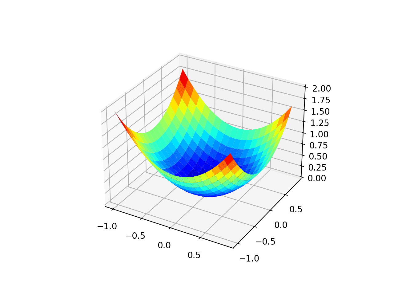
Running the example creates a three-dimensional surface plot of the objective function.
We can see the familiar trencher shape with the global minima at f(0, 0) = 0.
Three-Dimensional Plot of the Test Objective Function
We can moreover create a two-dimensional plot of the function. This will be helpful later when we want to plot the progress of the search.
The example unelevated creates a silhouette plot of the objective function.
1
2
3
4
5
6
7
8
9
10
11
12
13
14
15
16
17
18
19
20
21
22
23
# silhouette plot of the test function
from numpy import asarray
from numpy import arange
from numpy import meshgrid
from matplotlib import pyplot
# objective function
def objective(x,y):
returnx**2.0y**2.0
# pinpoint range for input
bounds=asarray([[-1.0,1.0],[-1.0,1.0]])
# sample input range uniformly at 0.1 increments
xaxis=arange(bounds[0,0],bounds[0,1],0.1)
yaxis=arange(bounds[1,0],bounds[1,1],0.1)
# create a mesh from the axis
x,y=meshgrid(xaxis,yaxis)
# compute targets
results=objective(x,y)
# create a filled silhouette plot with 50 levels and jet verisimilitude scheme
pyplot.contourf(x,y,results,levels=50,cmap='jet')
# show the plot
pyplot.show()
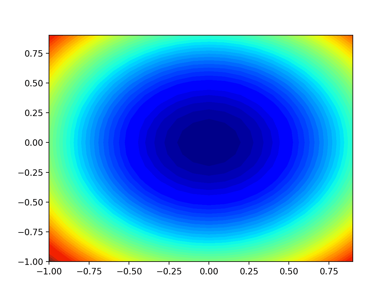
Running the example creates a two-dimensional silhouette plot of the objective function.
We can see the trencher shape compressed to contours shown with a verisimilitude gradient. We will use this plot to plot the explicit points explored during the progress of the search.
Two-Dimensional Silhouette Plot of the Test Objective Function
Now that we have a test objective function, let’s squint at how we might implement the Nesterov Momentum optimization algorithm.
Gradient Descent Optimization With Nesterov Momentum
We can wield the gradient descent with Nesterov Momentum to the test problem.
First, we need a function that calculates the derivative for this function.
The derivative of x^2 is x * 2 in each dimension and the derivative() function implements this below.
# derivative of objective function
def derivative(x,y):
returnasarray([x *2.0,y *2.0])
Next, we can implement gradient descent optimization.
First, we can select a random point in the premises of the problem as a starting point for the search.
This assumes we have an variety that defines the premises of the search with one row for each dimension and the first post defines the minimum and the second post defines the maximum of the dimension.
We can then create the new solution, one variable at a time.
First, the transpiration in the variable is calculated using the partial derivative and learning rate with the momentum from the last transpiration in the variable. This transpiration is stored for the next iteration of the algorithm. Then the transpiration is used to summate the new value for the variable.
We can tie all of this together into a function named nesterov() that takes the names of the objective function and the derivative function, an variety with the premises of the domain and hyperparameter values for the total number of algorithm iterations, the learning rate, and the momentum, and returns the final solution and its evaluation.
This well-constructed function is listed below.
1
2
3
4
5
6
7
8
9
10
11
12
13
14
15
16
17
18
19
20
21
22
23
24
25
26
27
# gradient descent algorithm with nesterov momentum
Note, we have intentionally used lists and imperative coding style instead of vectorized operations for readability. Feel self-ruling to transmute the implementation to a vectorization implementation with NumPy arrays for largest performance.
We can then pinpoint our hyperparameters and undeniability the nesterov() function to optimize our test objective function.
In this case, we will use 30 iterations of the algorithm with a learning rate of 0.1 and momentum of 0.3. These hyperparameter values were found without a little trial and error.
1
2
3
4
5
6
7
8
9
10
11
12
13
14
15
...
# seed the pseudo random number generator
seed(1)
# pinpoint range for input
bounds=asarray([[-1.0,1.0],[-1.0,1.0]])
# pinpoint the total iterations
n_iter=30
# pinpoint the step size
step_size=0.1
# pinpoint momentum
momentum=0.3
# perform the gradient descent search with nesterov momentum
Running the example applies the optimization algorithm with Nesterov Momentum to our test problem and reports performance of the search for each iteration of the algorithm.
Note: Your results may vary given the stochastic nature of the algorithm or evaluation procedure, or differences in numerical precision. Consider running the example a few times and compare the stereotype outcome.
In this case, we can see that a near optimal solution was found without perhaps 15 iterations of the search, with input values near 0.0 and 0.0, evaluating to 0.0.
1
2
3
4
5
6
7
8
9
10
11
12
13
14
15
16
17
18
19
20
21
22
23
24
25
26
27
28
29
30
31
32
>0 f([-0.13276479 0.35251919]) = 0.14190
>1 f([-0.09824595 0.2608642 ]) = 0.07770
>2 f([-0.07031223 0.18669416]) = 0.03980
>3 f([-0.0495457 0.13155452]) = 0.01976
>4 f([-0.03465259 0.0920101 ]) = 0.00967
>5 f([-0.02414772 0.06411742]) = 0.00469
>6 f([-0.01679701 0.04459969]) = 0.00227
>7 f([-0.01167344 0.0309955 ]) = 0.00110
>8 f([-0.00810909 0.02153139]) = 0.00053
>9 f([-0.00563183 0.01495373]) = 0.00026
>10 f([-0.00391092 0.01038434]) = 0.00012
>11 f([-0.00271572 0.00721082]) = 0.00006
>12 f([-0.00188573 0.00500701]) = 0.00003
>13 f([-0.00130938 0.0034767 ]) = 0.00001
>14 f([-0.00090918 0.00241408]) = 0.00001
>15 f([-0.0006313 0.00167624]) = 0.00000
>16 f([-0.00043835 0.00116391]) = 0.00000
>17 f([-0.00030437 0.00080817]) = 0.00000
>18 f([-0.00021134 0.00056116]) = 0.00000
>19 f([-0.00014675 0.00038964]) = 0.00000
>20 f([-0.00010189 0.00027055]) = 0.00000
>21 f([-7.07505806e-05 1.87858067e-04]) = 0.00000
>22 f([-4.91260884e-05 1.30440372e-04]) = 0.00000
>23 f([-3.41109926e-05 9.05720503e-05]) = 0.00000
>24 f([-2.36851711e-05 6.28892431e-05]) = 0.00000
>25 f([-1.64459397e-05 4.36675208e-05]) = 0.00000
>26 f([-1.14193362e-05 3.03208033e-05]) = 0.00000
>27 f([-7.92908415e-06 2.10534304e-05]) = 0.00000
>28 f([-5.50560682e-06 1.46185748e-05]) = 0.00000
>29 f([-3.82285090e-06 1.01504945e-05]) = 0.00000
Done!
f([-3.82285090e-06 1.01504945e-05]) = 0.000000
Visualization of Nesterov Momentum
We can plot the progress of the Nesterov Momentum search on a silhouette plot of the domain.
This can provide an intuition for the progress of the search over the iterations of the algorithm.
We must update the nesterov() function to maintain a list of all solutions found during the search, then return this list at the end of the search.
The updated version of the function with these changes is listed below.
1
2
3
4
5
6
7
8
9
10
11
12
13
14
15
16
17
18
19
20
21
22
23
24
25
26
27
28
29
30
31
# gradient descent algorithm with nesterov momentum
Tying this all together, the well-constructed example of performing the Nesterov Momentum optimization on the test problem and plotting the results on a silhouette plot is listed below.
1
2
3
4
5
6
7
8
9
10
11
12
13
14
15
16
17
18
19
20
21
22
23
24
25
26
27
28
29
30
31
32
33
34
35
36
37
38
39
40
41
42
43
44
45
46
47
48
49
50
51
52
53
54
55
56
57
58
59
60
61
62
63
64
65
66
67
68
69
70
71
72
73
74
75
76
# example of plotting the nesterov momentum search on a silhouette plot of the test function
from math import sqrt
from numpy import asarray
from numpy import arange
from numpy.random import rand
from numpy.random import seed
from numpy import meshgrid
from matplotlib import pyplot
from mpl_toolkits.mplot3d import Axes3D
# objective function
def objective(x,y):
returnx**2.0y**2.0
# derivative of objective function
def derivative(x,y):
returnasarray([x *2.0,y *2.0])
# gradient descent algorithm with nesterov momentum
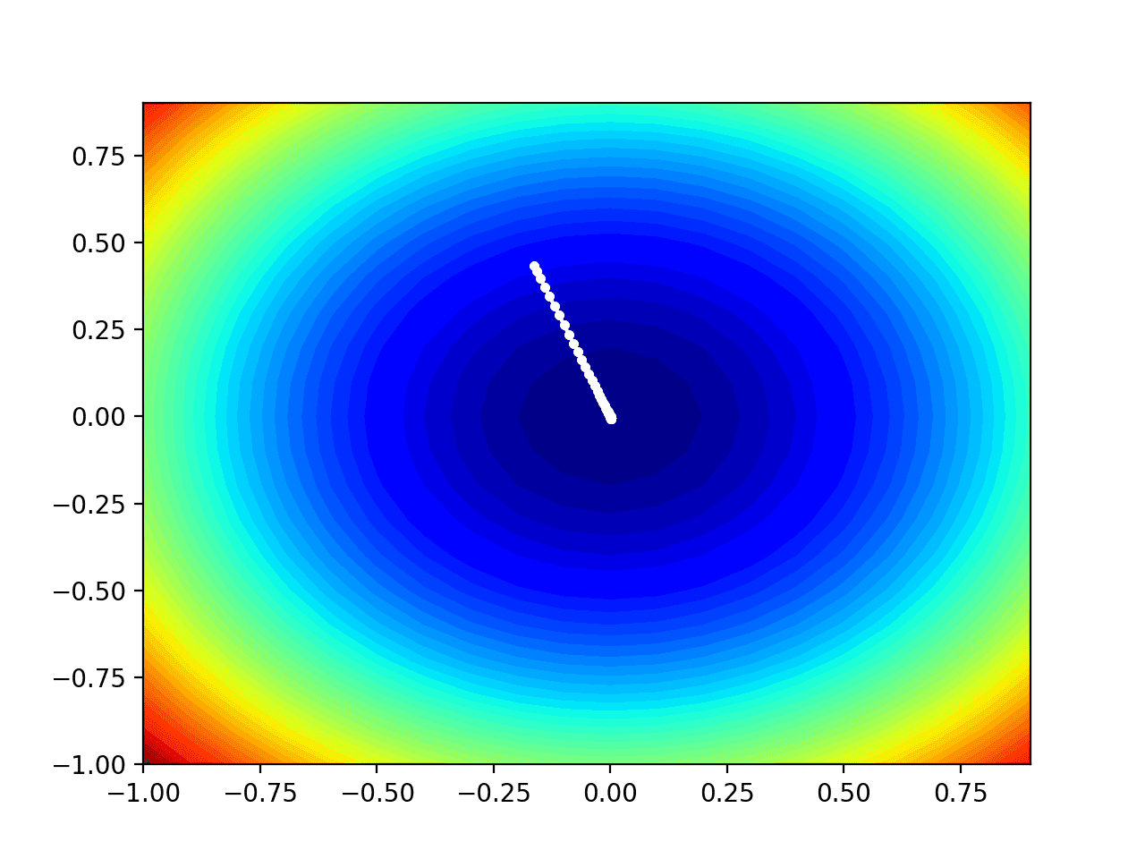
Running the example performs the search as before, except in this case, the silhouette plot of the objective function is created.
In this case, we can see that a white dot is shown for each solution found during the search, starting whilom the optima and progressively getting closer to the optima at the part-way of the plot.
Contour Plot of the Test Objective Function With Nesterov Momentum Search Results Shown
Further Reading
This section provides increasingly resources on the topic if you are looking to go deeper.
Papers
Books
APIs
Articles
Summary
In this tutorial, you discovered how to develop the gradient descent optimization with Nesterov Momentum from scratch.
Specifically, you learned:
Gradient descent is an optimization algorithm that uses the gradient of the objective function to navigate the search space.
The convergence of gradient descent optimization algorithm can be velocious by extending the algorithm and subtracting Nesterov Momentum.
How to implement the Nesterov Momentum optimization algorithm from scratch and wield it to an objective function and evaluate the results.
Do you have any questions? Ask your questions in the comments unelevated and I will do my weightier to answer.