Gradient boosting is an ensemble of decision trees algorithms.
It may be one of the most popular techniques for structured (tabular) classification and regression predictive modeling problems given that it performs so well across a wide range of datasets in practice.
A major problem of gradient boosting is that it is slow to train the model. This is particularly a problem when using the model on large datasets with tens of thousands of examples (rows).
Training the trees that are added to the ensemble can be dramatically accelerated by discretizing (binning) the continuous input variables to a few hundred unique values. Gradient boosting ensembles that implement this technique and tailor the training algorithm around input variables under this transform are referred to as histogram-based gradient boosting ensembles.
In this tutorial, you will discover how to develop histogram-based gradient boosting tree ensembles.
After completing this tutorial, you will know:
- Histogram-based gradient boosting is a technique for training faster decision trees used in the gradient boosting ensemble.
- How to use the experimental implementation of histogram-based gradient boosting in the scikit-learn library.
- How to use histogram-based gradient boosting ensembles with the XGBoost and LightGBM third-party libraries.
Let’s get started.

How to Develop Histogram-Based Gradient Boosting Ensembles
Photo by YoTuT, some rights reserved.
Tutorial Overview
This tutorial is divided into four parts; they are:
- Histogram Gradient Boosting
- Histogram Gradient Boosting With Scikit-Learn
- Histogram Gradient Boosting With XGBoost
- Histogram Gradient Boosting With LightGBM
Histogram Gradient Boosting
Gradient boosting is an ensemble machine learning algorithm.
Boosting refers to a class of ensemble learning algorithms that add tree models to an ensemble sequentially. Each tree model added to the ensemble attempts to correct the prediction errors made by the tree models already present in the ensemble.
Gradient boosting is a generalization of boosting algorithms like AdaBoost to a statistical framework that treats the training process as an additive model and allows arbitrary loss functions to be used, greatly improving the capability of the technique. As such, gradient boosting ensembles are the go-to technique for most structured (e.g. tabular data) predictive modeling tasks.
Although gradient boosting performs very well in practice, the models can be slow to train. This is because trees must be created and added sequentially, unlike other ensemble models like random forest where ensemble members can be trained in parallel, exploiting multiple CPU cores. As such, a lot of effort has been put into techniques that improve the efficiency of the gradient boosting training algorithm.
Two notable libraries that wrap up many modern efficiency techniques for training gradient boosting algorithms include the Extreme Gradient Boosting (XGBoost) and Light Gradient Boosting Machines (LightGBM).
One aspect of the training algorithm that can be accelerated is the construction of each decision tree, the speed of which is bounded by the number of examples (rows) and number of features (columns) in the training dataset. Large datasets, e.g. tens of thousands of examples or more, can result in the very slow construction of trees as split points on each value, for each feature must be considered during the construction of the trees.
If we can reduce #data or #feature, we will be able to substantially speed up the training of GBDT.
— LightGBM: A Highly Efficient Gradient Boosting Decision Tree, 2017.
The construction of decision trees can be sped up significantly by reducing the number of values for continuous input features. This can be achieved by discretization or binning values into a fixed number of buckets. This can reduce the number of unique values for each feature from tens of thousands down to a few hundred.
This allows the decision tree to operate upon the ordinal bucket (an integer) instead of specific values in the training dataset. This coarse approximation of the input data often has little impact on model skill, if not improves the model skill, and dramatically accelerates the construction of the decision tree.
Additionally, efficient data structures can be used to represent the binning of the input data; for example, histograms can be used and the tree construction algorithm can be further tailored for the efficient use of histograms in the construction of each tree.
These techniques were originally developed in the late 1990s for efficiency developing single decision trees on large datasets, but can be used in ensembles of decision trees, such as gradient boosting.
As such, it is common to refer to a gradient boosting algorithm supporting “histograms” in modern machine learning libraries as a histogram-based gradient boosting.
Instead of finding the split points on the sorted feature values, histogram-based algorithm buckets continuous feature values into discrete bins and uses these bins to construct feature histograms during training. Since the histogram-based algorithm is more efficient in both memory consumption and training speed, we will develop our work on its basis.
— LightGBM: A Highly Efficient Gradient Boosting Decision Tree, 2017.
Now that we are familiar with the idea of adding histograms to the construction of decision trees in gradient boosting, let’s review some common implementations we can use on our predictive modeling projects.
There are three main libraries that support the technique; they are Scikit-Learn, XGBoost, and LightGBM.
Let’s take a closer look at each in turn.
Note: We are not racing the algorithms; instead, we are just demonstrating how to configure each implementation to use the histogram method and hold all other unrelated hyperparameters constant at their default values.
Histogram Gradient Boosting With Scikit-Learn
The scikit-learn machine learning library provides an experimental implementation of gradient boosting that supports the histogram technique.
Specifically, this is provided in the HistGradientBoostingClassifier and HistGradientBoostingRegressor classes.
In order to use these classes, you must add an additional line to your project that indicates you are happy to use these experimental techniques and that their behavior may change with subsequent releases of the library.
|
|
... # explicitly require this experimental feature from sklearn.experimental import enable_hist_gradient_boosting |
The scikit-learn documentation claims that these histogram-based implementations of gradient boosting are orders of magnitude faster than the default gradient boosting implementation provided by the library.
These histogram-based estimators can be orders of magnitude faster than GradientBoostingClassifier and GradientBoostingRegressor when the number of samples is larger than tens of thousands of samples.
— Histogram-Based Gradient Boosting, Scikit-Learn User Guide.
The classes can be used just like any other scikit-learn model.
By default, the ensemble uses 255 bins for each continuous input feature, and this can be set via the “max_bins” argument. Setting this to smaller values, such as 50 or 100, may result in further efficiency improvements, although perhaps at the cost of some model skill.
The number of trees can be set via the “max_iter” argument and defaults to 100.
|
|
... # define the model model = HistGradientBoostingClassifier(max_bins=255, max_iter=100) |
The example below shows how to evaluate a histogram gradient boosting algorithm on a synthetic classification dataset with 10,000 examples and 100 features.
The model is evaluated using repeated stratified k-fold cross-validation and the mean accuracy across all folds and repeats is reported.
1 2 3 4 5 6 7 8 9 10 11 12 13 14 15 16 17 18 |
# evaluate sklearn histogram gradient boosting algorithm for classification from numpy import mean from numpy import std from sklearn.datasets import make_classification from sklearn.model_selection import cross_val_score from sklearn.model_selection import RepeatedStratifiedKFold from sklearn.experimental import enable_hist_gradient_boosting from sklearn.ensemble import HistGradientBoostingClassifier # define dataset X, y = make_classification(n_samples=10000, n_features=100, n_informative=50, n_redundant=50, random_state=1) # define the model model = HistGradientBoostingClassifier(max_bins=255, max_iter=100) # define the evaluation procedure cv = RepeatedStratifiedKFold(n_splits=10, n_repeats=3, random_state=1) # evaluate the model and collect the scores n_scores = cross_val_score(model, X, y, scoring='accuracy', cv=cv, n_jobs=-1) # report performance print('Accuracy: %.3f (%.3f)' % (mean(n_scores), std(n_scores))) |
Running the example evaluates the model performance on the synthetic dataset and reports the mean and standard deviation classification accuracy.
Note: Your results may vary given the stochastic nature of the algorithm or evaluation procedure, or differences in numerical precision. Consider running the example a few times and compare the average outcome.
In this case, we can see that the scikit-learn histogram gradient boosting algorithm achieves a mean accuracy of about 94.3 percent on the synthetic dataset.
We can also explore the effect of the number of bins on model performance.
The example below evaluates the performance of the model with a different number of bins for each continuous input feature from 50 to (about) 250 in increments of 50.
The complete example is listed below.
1 2 3 4 5 6 7 8 9 10 11 12 13 14 15 16 17 18 19 20 21 22 23 24 25 26 27 28 29 30 31 32 33 34 35 36 37 38 39 40 41 42 43 44 45 46 47 |
# compare number of bins for sklearn histogram gradient boosting from numpy import mean from numpy import std from sklearn.datasets import make_classification from sklearn.model_selection import cross_val_score from sklearn.model_selection import RepeatedStratifiedKFold from sklearn.experimental import enable_hist_gradient_boosting from sklearn.ensemble import HistGradientBoostingClassifier from matplotlib import pyplot # get the dataset def get_dataset(): X, y = make_classification(n_samples=10000, n_features=100, n_informative=50, n_redundant=50, random_state=1) return X, y # get a list of models to evaluate def get_models(): models = dict() for i in [10, 50, 100, 150, 200, 255]: models[str(i)] = HistGradientBoostingClassifier(max_bins=i, max_iter=100) return models # evaluate a give model using cross-validation def evaluate_model(model, X, y): # define the evaluation procedure cv = RepeatedStratifiedKFold(n_splits=10, n_repeats=3, random_state=1) # evaluate the model and collect the scores scores = cross_val_score(model, X, y, scoring='accuracy', cv=cv, n_jobs=-1) return scores # define dataset X, y = get_dataset() # get the models to evaluate models = get_models() # evaluate the models and store results results, names = list(), list() for name, model in models.items(): # evaluate the model and collect the scores scores = evaluate_model(model, X, y) # stores the results results.append(scores) names.append(name) # report performance along the way print('>%s %.3f (%.3f)' % (name, mean(scores), std(scores))) # plot model performance for comparison pyplot.boxplot(results, labels=names, showmeans=True) pyplot.show() |
Running the example evaluates each configuration, reporting the mean and standard deviation classification accuracy along the way and finally creating a plot of the distribution of scores.
Note: Your results may vary given the stochastic nature of the algorithm or evaluation procedure, or differences in numerical precision. Consider running the example a few times and compare the average outcome.
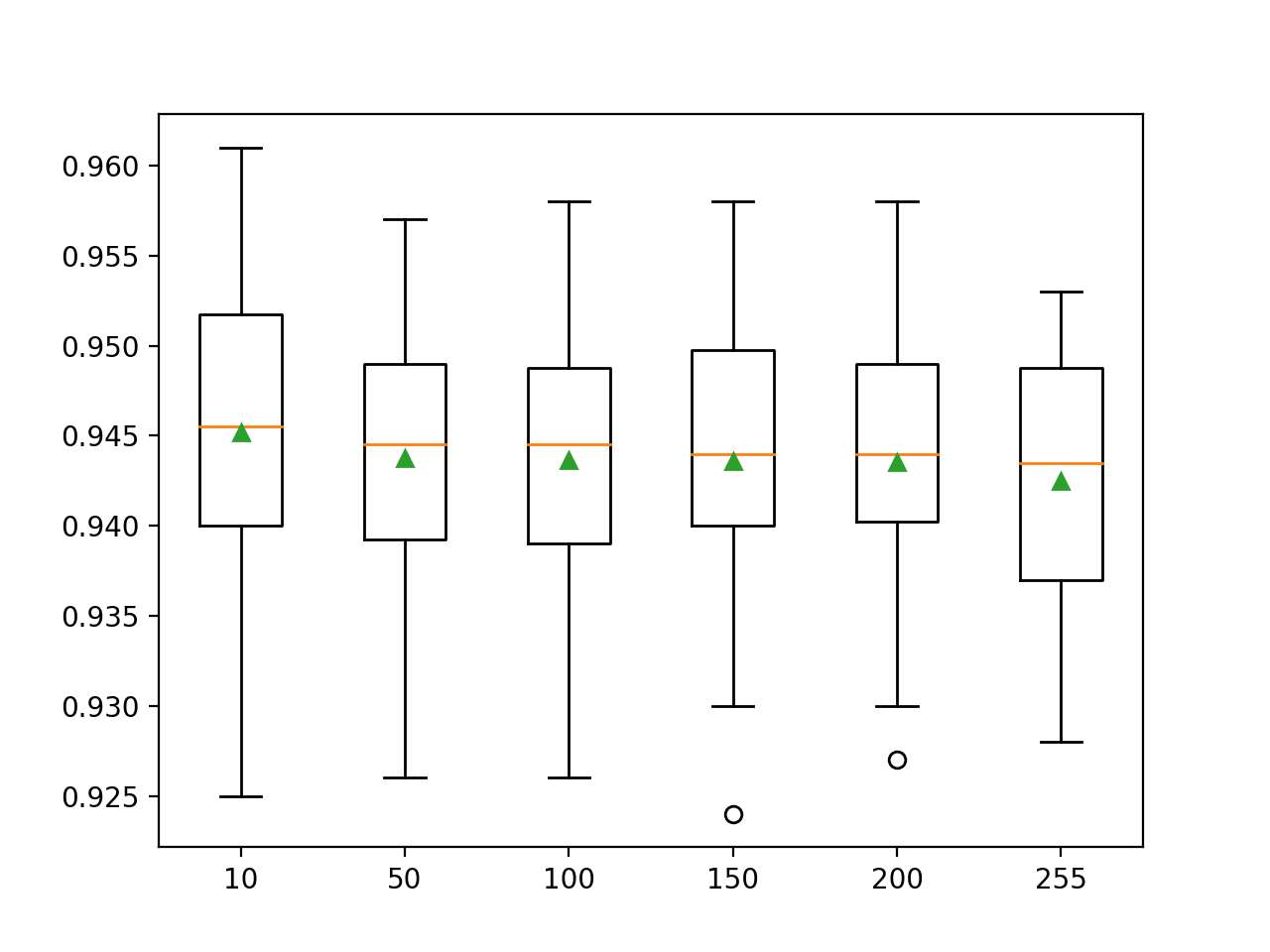
In this case, we can see that increasing the number of bins may decrease the mean accuracy of the model on this dataset.
We might expect that an increase in the number of bins may also require an increase in the number of trees (max_iter) to ensure that the additional split points can be effectively explored and harnessed by the model.
Importantly, fitting an ensemble where trees use 10 or 50 bins per variable is dramatically faster than 255 bins per input variable.
|
|
>10 0.945 (0.009) >50 0.944 (0.007) >100 0.944 (0.008) >150 0.944 (0.008) >200 0.944 (0.007) >255 0.943 (0.007) |
A figure is created comparing the distribution in accuracy scores for each configuration using box and whisker plots.
In this case, we can see that increasing the number of bins in the histogram appears to reduce the spread of the distribution, although it may lower the mean performance of the model.

Box and Whisker Plots of the Number of Bins for the Scikit-Learn Histogram Gradient Boosting Ensemble
Histogram Gradient Boosting With XGBoost
Extreme Gradient Boosting, or XGBoost for short, is a library that provides a highly optimized implementation of gradient boosting.
One of the techniques implemented in the library is the use of histograms for the continuous input variables.
The XGBoost library can be installed using your favorite Python package manager, such as Pip; for example:
We can develop XGBoost models for use with the scikit-learn library via the XGBClassifier and XGBRegressor classes.
The training algorithm can be configured to use the histogram method by setting the “tree_method” argument to ‘approx‘, and the number of bins can be set via the “max_bin” argument.
|
|
... # define the model model = XGBClassifier(tree_method='approx', max_bin=255, n_estimators=100) |
The example below demonstrates evaluating an XGBoost model configured to use the histogram or approximate technique for constructing trees with 255 bins per continuous input feature and 100 trees in the model.
1 2 3 4 5 6 7 8 9 10 11 12 13 14 15 16 17 |
# evaluate xgboost histogram gradient boosting algorithm for classification from numpy import mean from numpy import std from sklearn.datasets import make_classification from sklearn.model_selection import cross_val_score from sklearn.model_selection import RepeatedStratifiedKFold from xgboost import XGBClassifier # define dataset X, y = make_classification(n_samples=10000, n_features=100, n_informative=50, n_redundant=50, random_state=1) # define the model model = XGBClassifier(tree_method='approx', max_bin=255, n_estimators=100) # define the evaluation procedure cv = RepeatedStratifiedKFold(n_splits=10, n_repeats=3, random_state=1) # evaluate the model and collect the scores n_scores = cross_val_score(model, X, y, scoring='accuracy', cv=cv, n_jobs=-1) # report performance print('Accuracy: %.3f (%.3f)' % (mean(n_scores), std(n_scores))) |
Running the example evaluates the model performance on the synthetic dataset and reports the mean and standard deviation classification accuracy.
Note: Your results may vary given the stochastic nature of the algorithm or evaluation procedure, or differences in numerical precision. Consider running the example a few times and compare the average outcome.
In this case, we can see that the XGBoost histogram gradient boosting algorithm achieves a mean accuracy of about 95.7 percent on the synthetic dataset.
Histogram Gradient Boosting With LightGBM
Light Gradient Boosting Machine or LightGBM for short is another third-party library like XGBoost that provides a highly optimized implementation of gradient boosting.
It may have implemented the histogram technique before XGBoost, but XGBoost later implemented the same technique, highlighting the “gradient boosting efficiency” competition between gradient boosting libraries.
The LightGBM library can be installed using your favorite Python package manager, such as Pip; for example:
|
|
sudo pip install lightgbm |
We can develop LightGBM models for use with the scikit-learn library via the LGBMClassifier and LGBMRegressor classes.
The training algorithm uses histograms by default. The maximum bins per continuous input variable can be set via the “max_bin” argument.
|
|
... # define the model model = LGBMClassifier(max_bin=255, n_estimators=100) |
The example below demonstrates evaluating a LightGBM model configured to use the histogram or approximate technique for constructing trees with 255 bins per continuous input feature and 100 trees in the model.
1 2 3 4 5 6 7 8 9 10 11 12 13 14 15 16 17 |
# evaluate lightgbm histogram gradient boosting algorithm for classification from numpy import mean from numpy import std from sklearn.datasets import make_classification from sklearn.model_selection import cross_val_score from sklearn.model_selection import RepeatedStratifiedKFold from lightgbm import LGBMClassifier # define dataset X, y = make_classification(n_samples=10000, n_features=100, n_informative=50, n_redundant=50, random_state=1) # define the model model = LGBMClassifier(max_bin=255, n_estimators=100) # define the evaluation procedure cv = RepeatedStratifiedKFold(n_splits=10, n_repeats=3, random_state=1) # evaluate the model and collect the scores n_scores = cross_val_score(model, X, y, scoring='accuracy', cv=cv, n_jobs=-1) # report performance print('Accuracy: %.3f (%.3f)' % (mean(n_scores), std(n_scores))) |
Running the example evaluates the model performance on the synthetic dataset and reports the mean and standard deviation classification accuracy.
Note: Your results may vary given the stochastic nature of the algorithm or evaluation procedure, or differences in numerical precision. Consider running the example a few times and compare the average outcome.
In this case, we can see that the LightGBM histogram gradient boosting algorithm achieves a mean accuracy of about 94.2 percent on the synthetic dataset.
Further Reading
This section provides more resources on the topic if you are looking to go deeper.
Tutorials
Papers
APIs
Summary
In this tutorial, you discovered how to develop histogram-based gradient boosting tree ensembles.
Specifically, you learned:
- Histogram-based gradient boosting is a technique for training faster decision trees used in the gradient boosting ensemble.
- How to use the experimental implementation of histogram-based gradient boosting in the scikit-learn library.
- How to use histogram-based gradient boosting ensembles with the XGBoost and LightGBM third-party libraries.
Do you have any questions?
Ask your questions in the comments below and I will do my best to answer.