Tweet
Share
Share
Iterated Local Search is a stochastic global optimization algorithm.
It involves the repeated using of a local search algorithm
7k
By Nick Cotes
Iterated Local Search is a stochastic global optimization algorithm.
It involves the repeated using of a local search algorithm to modified versions of a good solution found previously. In this way, it is like a clever version of the stochastic hill climbing with random restarts algorithm.
The intuition overdue the algorithm is that random restarts can help to locate many local optima in a problem and that largest local optima are often tropical to other local optima. Therefore modest perturbations to existing local optima may locate largest or plane weightier solutions to an optimization problem.
In this tutorial, you will discover how to implement the iterated local search algorithm from scratch.
After completing this tutorial, you will know:
Iterated local search is a stochastic global search optimization algorithm that is a smarter version of stochastic hill climbing with random restarts.
How to implement stochastic hill climbing with random restarts from scratch.
How to implement and wield the iterated local search algorithm to a nonlinear objective function.
Let’s get started.
Iterated Local Search From Scratch in Python Photo by Susanne Nilsson, some rights reserved.
Tutorial Overview
This tutorial is divided into five parts; they are:
What Is Iterated Local Search
Ackley Objective Function
Stochastic Hill Climbing Algorithm
Stochastic Hill Climbing With Random Restarts
Iterated Local Search Algorithm
What Is Iterated Local Search
Iterated Local Search, or ILS for short, is a stochastic global search optimization algorithm.
It is related to or an extension of stochastic hill climbing and stochastic hill climbing with random starts.
It’s substantially a increasingly clever version of Hill-Climbing with Random Restarts.
Stochastic hill climbing is a local search algorithm that involves making random modifications to an existing solution and unsuspicious the modification only if it results in largest results than the current working solution.
Local search algorithms in unstipulated can get stuck in local optima. One tideway to write this problem is to restart the search from a new randomly selected starting point. The restart procedure can be performed many times and may be triggered without a stock-still number of function evaluations or if no remoter resurgence is seen for a given number of algorithm iterations. This algorithm is tabbed stochastic hill climbing with random restarts.
The simplest possibility to modernize upon a forfeit found by LocalSearch is to repeat the search from flipside starting point.
Iterated local search is similar to stochastic hill climbing with random restarts, except rather than selecting a random starting point for each restart, a point is selected based on a modified version of the weightier point found so far during the broader search.
The perturbation of the weightier solution so far is like a large jump in the search space to a new region, whereas the perturbations made by the stochastic hill climbing algorithm are much smaller, serving to a explicit region of the search space.
The heuristic here is that you can often find largest local optima near to the one you’re presently in, and walking from local optimum to local optimum in this way often outperforms just trying new locations entirely at random.
This allows the search to be performed at two levels. The hill climbing algorithm is the local search for getting the most out of a explicit candidate solution or region of the search space, and the restart tideway allows variegated regions of the search space to be explored.
In this way, the algorithm Iterated Local Search explores multiple local optima in the search space, increasing the likelihood of locating the global optima.
The Iterated Local Search was proposed for combinatorial optimization problems, such as the traveling salesman problem (TSP), although it can be unromantic to continuous function optimization by using variegated step sizes in the search space: smaller steps for the hill climbing and larger steps for the random restart.
Now that we are familiar with the Iterated Local Search algorithm, let’s explore how to implement the algorithm from scratch.
Ackley Objective Function
First, let’s pinpoint a channeling optimization problem as the understructure for implementing the Iterated Local Search algorithm.
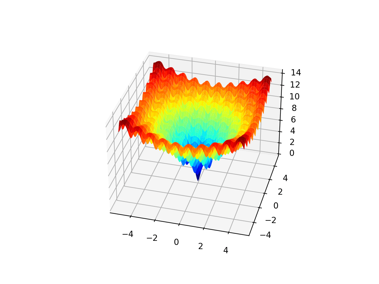
The Ackley function is an example of a multimodal objective function that has a each global optima and multiple local optima in which a local search might get stuck.
As such, a global optimization technique is required. It is a two-dimensional objective function that has a global optima at [0,0], which evaluates to 0.0.
The example unelevated implements the Ackley and creates a three-dimensional surface plot showing the global optima and multiple local optima.
# create a surface plot with the jet verisimilitude scheme
figure=pyplot.figure()
axis=figure.gca(projection='3d')
axis.plot_surface(x,y,results,cmap='jet')
# show the plot
pyplot.show()
Running the example creates the surface plot of the Ackley function showing the vast number of local optima.
3D Surface Plot of the Ackley Multimodal Function
We will use this as the understructure for implementing and comparing a simple stochastic hill climbing algorithm, stochastic hill climbing with random restarts, and finally iterated local search.
We would expect a stochastic hill climbing algorithm to get stuck hands in local minima. We would expect stochastic hill climbing with restarts to find many local minima, and we would expect iterated local search to perform largest than either method on this problem if configured appropriately.
Stochastic Hill Climbing Algorithm
Core to the Iterated Local Search algorithm is a local search, and in this tutorial, we will use the Stochastic Hill Climbing algorithm for this purpose.
The Stochastic Hill Climbing algorithm involves first generating a random starting point and current working solution, then generating perturbed versions of the current working solution and unsuspicious them if they are largest than the current working solution.
Given that we are working on a continuous optimization problem, a solution is a vector of values to be evaluated by the objective function, in this case, a point in a two-dimensional space regional by -5 and 5.
We can generate a random point by sampling the search space with a uniform probability distribution. For example:
We can generate perturbed versions of a currently working solution using a Gaussian probability distribution with the midpoint of the current values in the solution and a standard deviation controlled by a hyperparameter that controls how far the search is unliable to explore from the current working solution.
We will refer to this hyperparameter as “step_size“, for example:
...
# generate a perturbed version of a current working solution
candidate=solutionrandn(len(bounds))*step_size
Importantly, we must trammels that generated solutions are within the search space.
This can be achieved with a custom function named in_bounds() that takes a candidate solution and the premises of the search space and returns True if the point is in the search space, False otherwise.
# trammels if a point is within the premises of the search
def in_bounds(point,bounds):
# enumerate all dimensions of the point
fordinrange(len(bounds)):
# trammels if out of premises for this dimension
ifpoint[d]<bounds[d,0]orpoint[d]>bounds[d,1]:
returnFalse
returnTrue
This function can then be tabbed during the hill climb to personize that new points are in the premises of the search space, and if not, new points can be generated.
Tying this together, the function hillclimbing() unelevated implements the stochastic hill climbing local search algorithm. It takes the name of the objective function, premises of the problem, number of iterations, and steps size as arguments and returns the weightier solution and its evaluation.
We can test this algorithm on the Ackley function.
We will fix the seed for the pseudorandom number generator to ensure we get the same results each time the lawmaking is run.
The algorithm will be run for 1,000 iterations and a step size of 0.05 units will be used; both hyperparameters were chosen without a little trial and error.
At the end of the run, we will report the weightier solution found.
Running the example performs the stochastic hill climbing search on the objective function. Each resurgence found during the search is reported and the weightier solution is then reported at the end of the search.
Note: Your results may vary given the stochastic nature of the algorithm or evaluation procedure, or differences in numerical precision. Consider running the example a few times and compare the stereotype outcome.
In this case, we can see well-nigh 13 improvements during the search and a final solution of well-nigh f(-0.981, 1.965), resulting in an evaluation of well-nigh 5.381, which is far from f(0.0, 0.0) = 0.
1
2
3
4
5
6
7
8
9
10
11
12
13
14
15
>0 f([-0.85618854 2.1495965 ]) = 6.46986
>1 f([-0.81291816 2.03451957]) = 6.07149
>5 f([-0.82903902 2.01531685]) = 5.93526
>7 f([-0.83766043 1.97142393]) = 5.82047
>9 f([-0.89269139 2.02866012]) = 5.68283
>12 f([-0.8988359 1.98187164]) = 5.55899
>13 f([-0.9122303 2.00838942]) = 5.55566
>14 f([-0.94681334 1.98855174]) = 5.43024
>15 f([-0.98117198 1.94629146]) = 5.39010
>23 f([-0.97516403 1.97715161]) = 5.38735
>39 f([-0.98628044 1.96711371]) = 5.38241
>362 f([-0.9808789 1.96858459]) = 5.38233
>629 f([-0.98102417 1.96555308]) = 5.38194
Done!
f([-0.98102417 1.96555308]) = 5.381939
Next, we will modify the algorithm to perform random restarts and see if we can unzip largest results.
Stochastic Hill Climbing With Random Restarts
The Stochastic Hill Climbing With Random Restarts algorithm involves the repeated running of the Stochastic Hill Climbing algorithm and keeping track of the weightier solution found.
First, let’s modify the hillclimbing() function to take the starting point of the search rather than generating it randomly. This will help later when we implement the Iterated Local Search algorithm later.
We can then wield this algorithm to the Ackley objective function. In this case, we will limit the number of random restarts to 30, chosen arbitrarily.
The well-constructed example is listed below.
1
2
3
4
5
6
7
8
9
10
11
12
13
14
15
16
17
18
19
20
21
22
23
24
25
26
27
28
29
30
31
32
33
34
35
36
37
38
39
40
41
42
43
44
45
46
47
48
49
50
51
52
53
54
55
56
57
58
59
60
61
62
63
64
65
66
67
68
69
70
71
72
73
74
75
76
# hill climbing search with random restarts of the ackley objective function
Running the example will perform a stochastic hill climbing with random restarts search for the Ackley objective function. Each time an improved overall solution is discovered, it is reported and the final weightier solution found by the search is summarized.
Note: Your results may vary given the stochastic nature of the algorithm or evaluation procedure, or differences in numerical precision. Consider running the example a few times and compare the stereotype outcome.
In this case, we can see three improvements during the search and that the weightier solution found was approximately f(0.002, 0.002), which evaluated to well-nigh 0.009, which is much largest than a each run of the hill climbing algorithm.
Next, let’s squint at how we can implement the iterated local search algorithm.
Iterated Local Search Algorithm
The Iterated Local Search algorithm is a modified version of the stochastic hill climbing with random restarts algorithm.
The important difference is that the starting point for each using of the stochastic hill climbing algorithm is a perturbed version of the weightier point found so far.
We can implement this algorithm by using the random_restarts() function as a starting point. Each restart iteration, we can generate a modified version of the weightier solution found so far instead of a random starting point.
This can be achieved by using a step size hyperparameter, much like is used in the stochastic hill climber. In this case, a larger step size value will be used given the need for larger perturbations in the search space.
...
# generate an initial point as a perturbed version of the last best
We can then wield the algorithm to the Ackley objective function. In this case, we will use a larger step size value of 1.0 for the random restarts, chosen without a little trial and error.
The well-constructed example is listed below.
1
2
3
4
5
6
7
8
9
10
11
12
13
14
15
16
17
18
19
20
21
22
23
24
25
26
27
28
29
30
31
32
33
34
35
36
37
38
39
40
41
42
43
44
45
46
47
48
49
50
51
52
53
54
55
56
57
58
59
60
61
62
63
64
65
66
67
68
69
70
71
72
73
74
75
76
77
78
79
80
81
82
83
# iterated local search of the ackley objective function
Running the example will perform an Iterated Local Search of the Ackley objective function.
Each time an improved overall solution is discovered, it is reported and the final weightier solution found by the search is summarized at the end of the run.
Note: Your results may vary given the stochastic nature of the algorithm or evaluation procedure, or differences in numerical precision. Consider running the example a few times and compare the stereotype outcome.
In this case, we can see four improvements during the search and that the weightier solution found was two very small inputs that are tropical to zero, which evaluated to well-nigh 0.0003, which is largest than either a each run of the hill climber or the hill climber with restarts.