Method of Lagrange Multipliers: The Theory Behind Support Vector Machines (Part 3: Implementing An SVM From Scratch In Python)
Tweet
Share
Share
The mathematics that powers a support vector machine (SVM) classifier is beautiful. It is important to not only
5.1k
By Nick Cotes
The mathematics that powers a support vector machine (SVM) classifier is beautiful. It is important to not only learn the basic model of an SVM but also know how you can implement the entire model from scratch. This is a continuation of our series of tutorials on SVMs. In part1 and part2 of this series we discussed the mathematical model behind a linear SVM. In this tutorial, we’ll show how you can build an SVM linear classifier using the optimization routines shipped with Python’s SciPy library.
After completing this tutorial, you will know:
How to use SciPy’s optimization routines
How to define the objective function
How to define bounds and linear constraints
How to implement your own SVM classifier in Python
Let’s get started.
Method Of Lagrange Multipliers: The Theory Behind Support Vector Machines (Part 3: Implementing An SVM From Scratch In Python) Sculpture Gyre by Thomas Sayre, Photo by Mehreen Saeed, some rights reserved.
Tutorial Overview
This tutorial is divided into 2 parts; they are:
The optimization problem of an SVM
Solution of the optimization problem in Python
Define the objective function
Define the bounds and linear constraints
Solve the problem with different C values
Pre-requisites
For this tutorial, it is assumed that you are already familiar with the following topics. You can click on the individual links to get more details.
Notations and Assumptions
A basic SVM machine assumes a binary classification problem. Suppose, we have $m$ training points, each point being an $n$-dimensional vector. We’ll use the following notations:
$m$: Total training points
$n$: Dimensionality of each training point
$x$: Data point, which is an $n$-dimensional vector
$i$: Subscript used to index the training points. $0 leq i < m$
$k$: Subscript used to index the training points. $0 leq k < m$
$j$: Subscript used to index each dimension of a training point
$t$: Label of a data point. It is an $m$-dimensional vector, with $t_i in {-1, +1}$
$T$: Transpose operator
$w$: Weight vector denoting the coefficients of the hyperplane. It is also an $n$-dimensional vector
$alpha$: Vector of Lagrange multipliers, also an $m$-dimensional vector
$C$: User defined penalty factor/regularization constant
The SVM Optimization Problem
The SVM classifier maximizes the following Lagrange dual given by: $$ L_d = -frac{1}{2} sum_i sum_k alpha_i alpha_k t_i t_k (x_i)^T (x_k) + sum_i alpha_i $$
The above function is subject to the following constraints:
We also need the following constant to detect all alphas numerically close to zero, so we need to define our own threshold for zero.
ZERO=1e-7
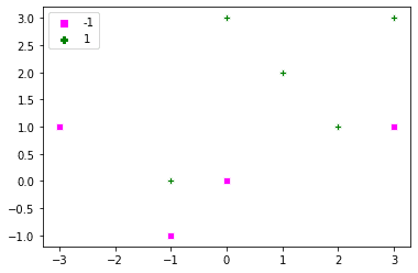
Defining the Data Points and Labels
Let’s define a very simple dataset, the corresponding labels and a simple routine for plotting this data. Optionally, if a string of alphas is given to the plotting function, then it will also label all support vectors with their corresponding alpha values. Just to recall support vectors are those points for which $alpha>0$.
Let’s look at the minimize() function in scipy.optimize library. It requires the following arguments:
The objective function to minimize. Lagrange dual in our case.
The initial values of variables with respect to which the minimization takes place. In this problem, we have to determine the Lagrange multipliers $alpha$. We’ll initialize all $alpha$ randomly.
The method to use for optimization. We’ll use trust-constr.
The linear constraints on $alpha$.
The bounds on $alpha$.
Defining the Objective Function
Our objective function is $L_d$ defined above, which has to be maximized. As we are using the minimize() function, we have to multiply $L_d$ by (-1) to maximize it. Its implementation is given below. The first parameter for the objective function is the variable w.r.t. which the optimization takes place. We also need the training points and the corresponding labels as additional arguments.
You can shorten the code for the lagrange_dual() function given below by using matrices. However, in this tutorial, it is kept very simple to make everything clear.
Let’s write the overall routine to find the optimal values of alpha when given the parameters x, t, and C. The objective function requires the additional arguments x and t, which are passed via args in minimize().
The expression for the hyperplane is given by: $$ w^T x + w_0 = 0 $$
For the hyperplane, we need the weight vector $w$ and the constant $w_0$. The weight vector is given by: $$ w = sum_i alpha_i t_i x_i $$
If there are too many training points, it’s best to use only support vectors with $alpha>0$ to compute the weight vector.
For $w_0$, we’ll compute it from each support vector $s$, for which $alpha_s < C$, and then take the average. For a single support vector $x_s$, $w_0$ is given by:
$$ w_0 = t_s – w^T x_s $$
A support vector’s alpha cannot be numerically exactly equal to C. Hence, we can subtract a small constant from C to find all support vectors with $alpha_s < C$. This is done in the get_w0() function.
Let’s write the corresponding function that can take as argument an array of test points along with $w$ and $w_0$ and classify various points. We have also added a second function for calculating the misclassification rate:
1
2
3
4
5
6
7
8
9
10
11
12
defclassify_points(x_test,w,w0):
# get y(x_test)
predicted_labels=np.sum(x_test*w,axis=1)+w0
predicted_labels=np.sign(predicted_labels)
# Assign a label arbitrarily a +1 if it is zero
predicted_labels[predicted_labels==0]=1
returnpredicted_labels
defmisclassification_rate(labels,predictions):
total=len(labels)
errors=sum(labels!=predictions)
returnerrors/total*100
Plotting the Margin and Hyperplane
Let’s also define functions to plot the hyperplane and the soft margin.
1
2
3
4
5
6
7
8
9
10
11
defplot_hyperplane(w,w0):
x_coord=np.array(plt.gca().get_xlim())
y_coord=-w0/w[1]-w[0]/w[1]*x_coord
plt.plot(x_coord,y_coord,color='red')
defplot_margin(w,w0):
x_coord=np.array(plt.gca().get_xlim())
ypos_coord=1/w[1]-w0/w[1]-w[0]/w[1]*x_coord
plt.plot(x_coord,ypos_coord,'--',color='green')
yneg_coord=-1/w[1]-w0/w[1]-w[0]/w[1]*x_coord
plt.plot(x_coord,yneg_coord,'--',color='magenta')
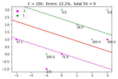
Powering Up The SVM
It’s now time to run the SVM. The function display_SVM_result() will help us visualize everything. We’ll initialize alpha to random values, define C and find the best values of alpha in this function. We’ll also plot the hyperplane, the margin and the data points. The support vectors would also be labelled by their corresponding alpha value. The title of the plot would be the percentage of errors and number of support vectors.
1
2
3
4
5
6
7
8
9
10
11
12
13
14
15
16
17
18
19
20
21
22
defdisplay_SVM_result(x,t,C):
# Get the alphas
alpha=optimize_alpha(x,t,C)
# Get the weights
w=get_w(alpha,t,x)
w0=get_w0(alpha,t,x,w,C)
plot_x(x,t,alpha,C)
xlim=plt.gca().get_xlim()
ylim=plt.gca().get_ylim()
plot_hyperplane(w,w0)
plot_margin(w,w0)
plt.xlim(xlim)
plt.ylim(ylim)
# Get the misclassification error and display it as title
title=title+', total SV = '+str(len(alpha[alpha>ZERO]))
plt.title(title)
display_SVM_result(dat,labels,100)
plt.show()
The Effect of C
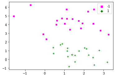
If you change the value of C to $infty$, then the soft margin turns into a hard margin, with no toleration for errors. The problem we defined above is not solvable in this case. Let’s generate an artificial set of points and look at the effect of C on classification. To understand the entire problem, we’ll use a simple dataset, where the positive and negative examples are separable.
Below are the points generated via make_blobs():
dat,labels=dt.make_blobs(n_samples=[20,20],
cluster_std=1,
random_state=0)
labels[labels==0]=-1
plot_x(dat,labels)
Now let’s define different values of C and run the code.
fig=plt.figure(figsize=(8,25))
i=0
C_array=[1e-2,100,1e5]
forCinC_array:
fig.add_subplot(311+i)
display_SVM_result(dat,labels,C)
i=i+1
Comments on the Result
The above is a nice example, which shows that increasing $C$, decreases the margin. A high value of $C$ adds a stricter penalty on errors. A smaller value allows a wider margin and more misclassification errors. Hence, $C$ defines a tradeoff between the maximization of margin and classification errors.
Consolidated Code
Here is the consolidated code, that you can paste in your Python file and run it at your end. You can experiment with different values of $C$ and try out the different optimization methods given as arguments to the minimize() function.


 Comments on the Result