Multinomial Logistic Regression With Python || Blockchain & Web development

Multinomial logistic regression is an extension of logistic regression that adds native support for multi-class classification problems.

Logistic regression, by default, is limited to two-class classification problems. Some extensions like one-vs-rest can allow logistic regression to be used for multi-class classification problems, although they require that the classification problem first be transformed into multiple binary classification problems.

Instead, the multinomial logistic regression algorithm is an extension to the logistic regression model that involves changing the loss function to cross-entropy loss and predict probability distribution to a multinomial probability distribution to natively support multi-class classification problems.

In this tutorial, you will discover how to develop multinomial logistic regression models in Python.

After completing this tutorial, you will know:

Multinomial logistic regression is an extension of logistic regression for multi-class classification.
How to develop and evaluate multinomial logistic regression and develop a final model for making predictions on new data.
How to tune the penalty hyperparameter for the multinomial logistic regression model.

Let’s get started.

Multinomial Logistic Regression With Python
Photo by Nicolas Rénac, some rights reserved.

Tutorial Overview

This tutorial is divided into three parts; they are:

Multinomial Logistic Regression
Evaluate Multinomial Logistic Regression Model
Tune Penalty for Multinomial Logistic Regression

Multinomial Logistic Regression

Logistic regression is a classification algorithm.

It is intended for datasets that have numerical input variables and a categorical target variable that has two values or classes. Problems of this type are referred to as binary classification problems.

Logistic regression is designed for two-class problems, modeling the target using a binomial probability distribution function. The class labels are mapped to 1 for the positive class or outcome and 0 for the negative class or outcome. The fit model predicts the probability that an example belongs to class 1.

By default, logistic regression cannot be used for classification tasks that have more than two class labels, so-called multi-class classification.

Instead, it requires modification to support multi-class classification problems.

One popular approach for adapting logistic regression to multi-class classification problems is to split the multi-class classification problem into multiple binary classification problems and fit a standard logistic regression model on each subproblem. Techniques of this type include one-vs-rest and one-vs-one wrapper models.

An alternate approach involves changing the logistic regression model to support the prediction of multiple class labels directly. Specifically, to predict the probability that an input example belongs to each known class label.

The probability distribution that defines multi-class probabilities is called a multinomial probability distribution. A logistic regression model that is adapted to learn and predict a multinomial probability distribution is referred to as Multinomial Logistic Regression. Similarly, we might refer to default or standard logistic regression as Binomial Logistic Regression.

Binomial Logistic Regression: Standard logistic regression that predicts a binomial probability (i.e. for two classes) for each input example.
Multinomial Logistic Regression: Modified version of logistic regression that predicts a multinomial probability (i.e. more than two classes) for each input example.

If you are new to binomial and multinomial probability distributions, you may want to read the tutorial:

Changing logistic regression from binomial to multinomial probability requires a change to the loss function used to train the model (e.g. log loss to cross-entropy loss), and a change to the output from a single probability value to one probability for each class label.

Now that we are familiar with multinomial logistic regression, let’s look at how we might develop and evaluate multinomial logistic regression models in Python.

Evaluate Multinomial Logistic Regression Model

In this section, we will develop and evaluate a multinomial logistic regression model using the scikit-learn Python machine learning library.

First, we will define a synthetic multi-class classification dataset to use as the basis of the investigation. This is a generic dataset that you can easily replace with your own loaded dataset later.

The make_classification() function can be used to generate a dataset with a given number of rows, columns, and classes. In this case, we will generate a dataset with 1,000 rows, 10 input variables or columns, and 3 classes.

The example below generates the dataset and summarizes the shape of the arrays and the distribution of examples across the three classes.

# test classification dataset from collections import Counter from sklearn.datasets import make_classification # define dataset X, y = make_classification(n_samples=1000, n_features=10, n_informative=5, n_redundant=5, n_classes=3, random_state=1) # summarize the dataset print(X.shape, y.shape) print(Counter(y))

# test classification dataset

from collections import Counter

from sklearn.datasets import make_classification

# define dataset

X, y = make_classification(n_samples=1000, n_features=10, n_informative=5, n_redundant=5, n_classes=3, random_state=1)

# summarize the dataset

print(X.shape, y.shape)

print(Counter(y))

Running the example confirms that the dataset has 1,000 rows and 10 columns, as we expected, and that the rows are distributed approximately evenly across the three classes, with about 334 examples in each class.

(1000, 10) (1000,) Counter({1: 334, 2: 334, 0: 332})

(1000, 10) (1000,)

Counter({1: 334, 2: 334, 0: 332})

Logistic regression is supported in the scikit-learn library via the LogisticRegression class.

The LogisticRegression class can be configured for multinomial logistic regression by setting the “multi_class” argument to “multinomial” and the “solver” argument to a solver that supports multinomial logistic regression, such as “lbfgs“.

... # define the multinomial logistic regression model model = LogisticRegression(multi_class='multinomial', solver='lbfgs')

...

# define the multinomial logistic regression model

model = LogisticRegression(multi_class='multinomial', solver='lbfgs')

The multinomial logistic regression model will be fit using cross-entropy loss and will predict the integer value for each integer encoded class label.

Now that we are familiar with the multinomial logistic regression API, we can look at how we might evaluate a multinomial logistic regression model on our synthetic multi-class classification dataset.

It is a good practice to evaluate classification models using repeated stratified k-fold cross-validation. The stratification ensures that each cross-validation fold has approximately the same distribution of examples in each class as the whole training dataset.

We will use three repeats with 10 folds, which is a good default, and evaluate model performance using classification accuracy given that the classes are balanced.

The complete example of evaluating multinomial logistic regression for multi-class classification is listed below.

# evaluate multinomial logistic regression model from numpy import mean from numpy import std from sklearn.datasets import make_classification from sklearn.model_selection import cross_val_score from sklearn.model_selection import RepeatedStratifiedKFold from sklearn.linear_model import LogisticRegression # define dataset X, y = make_classification(n_samples=1000, n_features=10, n_informative=5, n_redundant=5, n_classes=3, random_state=1) # define the multinomial logistic regression model model = LogisticRegression(multi_class='multinomial', solver='lbfgs') # define the model evaluation procedure cv = RepeatedStratifiedKFold(n_splits=10, n_repeats=3, random_state=1) # evaluate the model and collect the scores n_scores = cross_val_score(model, X, y, scoring='accuracy', cv=cv, n_jobs=-1) # report the model performance print('Mean Accuracy: %.3f (%.3f)' % (mean(n_scores), std(n_scores)))

# evaluate multinomial logistic regression model

from numpy import mean

from numpy import std

from sklearn.datasets import make_classification

from sklearn.model_selection import cross_val_score

from sklearn.model_selection import RepeatedStratifiedKFold

from sklearn.linear_model import LogisticRegression

# define dataset

X, y = make_classification(n_samples=1000, n_features=10, n_informative=5, n_redundant=5, n_classes=3, random_state=1)

# define the multinomial logistic regression model

model = LogisticRegression(multi_class='multinomial', solver='lbfgs')

# define the model evaluation procedure

cv = RepeatedStratifiedKFold(n_splits=10, n_repeats=3, random_state=1)

# evaluate the model and collect the scores

n_scores = cross_val_score(model, X, y, scoring='accuracy', cv=cv, n_jobs=-1)

# report the model performance

print('Mean Accuracy: %.3f (%.3f)' % (mean(n_scores), std(n_scores)))

Running the example reports the mean classification accuracy across all folds and repeats of the evaluation procedure.

Note: Your results may vary given the stochastic nature of the algorithm or evaluation procedure, or differences in numerical precision. Consider running the example a few times and compare the average outcome.

In this case, we can see that the multinomial logistic regression model with default penalty achieved a mean classification accuracy of about 68.1 percent on our synthetic classification dataset.

Mean Accuracy: 0.681 (0.042)

We may decide to use the multinomial logistic regression model as our final model and make predictions on new data.

This can be achieved by first fitting the model on all available data, then calling the predict() function to make a prediction for new data.

The example below demonstrates how to make a prediction for new data using the multinomial logistic regression model.

# make a prediction with a multinomial logistic regression model from sklearn.datasets import make_classification from sklearn.linear_model import LogisticRegression # define dataset X, y = make_classification(n_samples=1000, n_features=10, n_informative=5, n_redundant=5, n_classes=3, random_state=1) # define the multinomial logistic regression model model = LogisticRegression(multi_class='multinomial', solver='lbfgs') # fit the model on the whole dataset model.fit(X, y) # define a single row of input data row = [1.89149379, -0.39847585, 1.63856893, 0.01647165, 1.51892395, -3.52651223, 1.80998823, 0.58810926, -0.02542177, -0.52835426] # predict the class label yhat = model.predict([row]) # summarize the predicted class print('Predicted Class: %d' % yhat[0])

# make a prediction with a multinomial logistic regression model

from sklearn.datasets import make_classification

from sklearn.linear_model import LogisticRegression

# define dataset

X, y = make_classification(n_samples=1000, n_features=10, n_informative=5, n_redundant=5, n_classes=3, random_state=1)

# define the multinomial logistic regression model

model = LogisticRegression(multi_class='multinomial', solver='lbfgs')

# fit the model on the whole dataset

model.fit(X, y)

# define a single row of input data

row = [1.89149379, -0.39847585, 1.63856893, 0.01647165, 1.51892395, -3.52651223, 1.80998823, 0.58810926, -0.02542177, -0.52835426]

# predict the class label

yhat = model.predict([row])

# summarize the predicted class

print('Predicted Class: %d' % yhat[0])

Running the example first fits the model on all available data, then defines a row of data, which is provided to the model in order to make a prediction.

In this case, we can see that the model predicted the class “1” for the single row of data.

Predicted Class: 1

A benefit of multinomial logistic regression is that it can predict calibrated probabilities across all known class labels in the dataset.

This can be achieved by calling the predict_proba() function on the model.

The example below demonstrates how to predict a multinomial probability distribution for a new example using the multinomial logistic regression model.

# predict probabilities with a multinomial logistic regression model from sklearn.datasets import make_classification from sklearn.linear_model import LogisticRegression # define dataset X, y = make_classification(n_samples=1000, n_features=10, n_informative=5, n_redundant=5, n_classes=3, random_state=1) # define the multinomial logistic regression model model = LogisticRegression(multi_class='multinomial', solver='lbfgs') # fit the model on the whole dataset model.fit(X, y) # define a single row of input data row = [1.89149379, -0.39847585, 1.63856893, 0.01647165, 1.51892395, -3.52651223, 1.80998823, 0.58810926, -0.02542177, -0.52835426] # predict a multinomial probability distribution yhat = model.predict_proba([row]) # summarize the predicted probabilities print('Predicted Probabilities: %s' % yhat[0])

# predict probabilities with a multinomial logistic regression model

from sklearn.datasets import make_classification

from sklearn.linear_model import LogisticRegression

# define dataset

X, y = make_classification(n_samples=1000, n_features=10, n_informative=5, n_redundant=5, n_classes=3, random_state=1)

# define the multinomial logistic regression model

model = LogisticRegression(multi_class='multinomial', solver='lbfgs')

# fit the model on the whole dataset

model.fit(X, y)

# define a single row of input data

row = [1.89149379, -0.39847585, 1.63856893, 0.01647165, 1.51892395, -3.52651223, 1.80998823, 0.58810926, -0.02542177, -0.52835426]

# predict a multinomial probability distribution

yhat = model.predict_proba([row])

# summarize the predicted probabilities

print('Predicted Probabilities: %s' % yhat[0])

Running the example first fits the model on all available data, then defines a row of data, which is provided to the model in order to predict class probabilities.

In this case, we can see that class 1 (e.g. the array index is mapped to the class integer value) has the largest predicted probability with about 0.50.

Predicted Probabilities: [0.16470456 0.50297138 0.33232406]

Now that we are familiar with evaluating and using multinomial logistic regression models, let’s explore how we might tune the model hyperparameters.

Tune Penalty for Multinomial Logistic Regression

An important hyperparameter to tune for multinomial logistic regression is the penalty term.

This term imposes pressure on the model to seek smaller model weights. This is achieved by adding a weighted sum of the model coefficients to the loss function, encouraging the model to reduce the size of the weights along with the error while fitting the model.

A popular type of penalty is the L2 penalty that adds the (weighted) sum of the squared coefficients to the loss function. A weighting of the coefficients can be used that reduces the strength of the penalty from full penalty to a very slight penalty.

By default, the LogisticRegression class uses the L2 penalty with a weighting of coefficients set to 1.0. The type of penalty can be set via the “penalty” argument with values of “l1“, “l2“, “elasticnet” (e.g. both), although not all solvers support all penalty types. The weighting of the coefficients in the penalty can be set via the “C” argument.

... # define the multinomial logistic regression model with a default penalty LogisticRegression(multi_class='multinomial', solver='lbfgs', penalty='l2', C=1.0)

...

# define the multinomial logistic regression model with a default penalty

LogisticRegression(multi_class='multinomial', solver='lbfgs', penalty='l2', C=1.0)

The weighting for the penalty is actually the inverse weighting, perhaps penalty = 1 – C.

From the documentation:

C : float, default=1.0
Inverse of regularization strength; must be a positive float. Like in support vector machines, smaller values specify stronger regularization.

This means that values close to 1.0 indicate very little penalty and values close to zero indicate a strong penalty. A C value of 1.0 may indicate no penalty at all.

C close to 1.0: Light penalty.
C close to 0.0: Strong penalty.

The penalty can be disabled by setting the “penalty” argument to the string “none“.

... # define the multinomial logistic regression model without a penalty LogisticRegression(multi_class='multinomial', solver='lbfgs', penalty='none')

...

# define the multinomial logistic regression model without a penalty

LogisticRegression(multi_class='multinomial', solver='lbfgs', penalty='none')

Now that we are familiar with the penalty, let’s look at how we might explore the effect of different penalty values on the performance of the multinomial logistic regression model.

It is common to test penalty values on a log scale in order to quickly discover the scale of penalty that works well for a model. Once found, further tuning at that scale may be beneficial.

We will explore the L2 penalty with weighting values in the range from 0.0001 to 1.0 on a log scale, in addition to no penalty or 0.0.

The complete example of evaluating L2 penalty values for multinomial logistic regression is listed below.

# tune regularization for multinomial logistic regression from numpy import mean from numpy import std from sklearn.datasets import make_classification from sklearn.model_selection import cross_val_score from sklearn.model_selection import RepeatedStratifiedKFold from sklearn.linear_model import LogisticRegression from matplotlib import pyplot # get the dataset def get_dataset(): X, y = make_classification(n_samples=1000, n_features=20, n_informative=15, n_redundant=5, random_state=1, n_classes=3) return X, y # get a list of models to evaluate def get_models(): models = dict() for p in [0.0, 0.0001, 0.001, 0.01, 0.1, 1.0]: # create name for model key = '%.4f' % p # turn off penalty in some cases if p == 0.0: # no penalty in this case models[key] = LogisticRegression(multi_class='multinomial', solver='lbfgs', penalty='none') else: models[key] = LogisticRegression(multi_class='multinomial', solver='lbfgs', penalty='l2', C=p) return models # evaluate a give model using cross-validation def evaluate_model(model, X, y): # define the evaluation procedure cv = RepeatedStratifiedKFold(n_splits=10, n_repeats=3, random_state=1) # evaluate the model scores = cross_val_score(model, X, y, scoring='accuracy', cv=cv, n_jobs=-1) return scores # define dataset X, y = get_dataset() # get the models to evaluate models = get_models() # evaluate the models and store results results, names = list(), list() for name, model in models.items(): # evaluate the model and collect the scores scores = evaluate_model(model, X, y) # store the results results.append(scores) names.append(name) # summarize progress along the way print('>%s %.3f (%.3f)' % (name, mean(scores), std(scores))) # plot model performance for comparison pyplot.boxplot(results, labels=names, showmeans=True) pyplot.show()

# tune regularization for multinomial logistic regression

from numpy import mean

from numpy import std

from sklearn.datasets import make_classification

from sklearn.model_selection import cross_val_score

from sklearn.model_selection import RepeatedStratifiedKFold

from sklearn.linear_model import LogisticRegression

from matplotlib import pyplot

# get the dataset

def get_dataset():

X, y = make_classification(n_samples=1000, n_features=20, n_informative=15, n_redundant=5, random_state=1, n_classes=3)

return X, y

# get a list of models to evaluate

def get_models():

models = dict()

for p in [0.0, 0.0001, 0.001, 0.01, 0.1, 1.0]:

# create name for model

key = '%.4f' % p

# turn off penalty in some cases

if p == 0.0:

# no penalty in this case

models[key] = LogisticRegression(multi_class='multinomial', solver='lbfgs', penalty='none')

else:

models[key] = LogisticRegression(multi_class='multinomial', solver='lbfgs', penalty='l2', C=p)

return models

# evaluate a give model using cross-validation

def evaluate_model(model, X, y):

# define the evaluation procedure

cv = RepeatedStratifiedKFold(n_splits=10, n_repeats=3, random_state=1)

# evaluate the model

scores = cross_val_score(model, X, y, scoring='accuracy', cv=cv, n_jobs=-1)

return scores

# define dataset

X, y = get_dataset()

# get the models to evaluate

models = get_models()

# evaluate the models and store results

results, names = list(), list()

for name, model in models.items():

# evaluate the model and collect the scores

scores = evaluate_model(model, X, y)

# store the results

results.append(scores)

names.append(name)

# summarize progress along the way

print('>%s %.3f (%.3f)' % (name, mean(scores), std(scores)))

# plot model performance for comparison

pyplot.boxplot(results, labels=names, showmeans=True)

pyplot.show()

Running the example reports the mean classification accuracy for each configuration along the way.

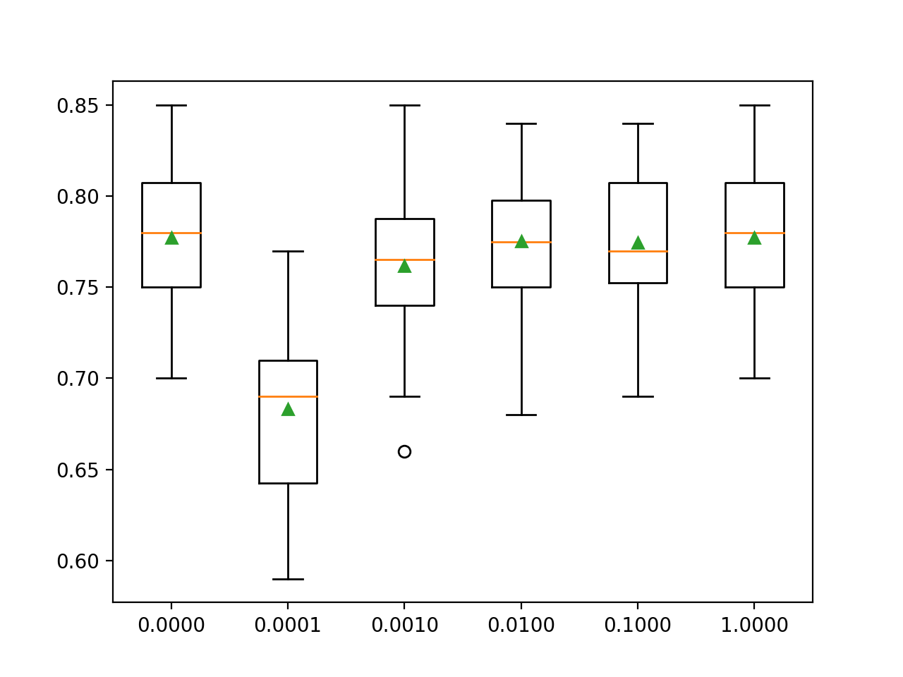
In this case, we can see that a C value of 1.0 has the best score of about 77.7 percent, which is the same as using no penalty that achieves the same score.

>0.0000 0.777 (0.037) >0.0001 0.683 (0.049) >0.0010 0.762 (0.044) >0.0100 0.775 (0.040) >0.1000 0.774 (0.038) >1.0000 0.777 (0.037)

>0.0000 0.777 (0.037)

>0.0001 0.683 (0.049)

>0.0010 0.762 (0.044)

>0.0100 0.775 (0.040)

>0.1000 0.774 (0.038)

>1.0000 0.777 (0.037)

A box and whisker plot is created for the accuracy scores for each configuration and all plots are shown side by side on a figure on the same scale for direct comparison.

In this case, we can see that the larger penalty we use on this dataset (i.e. the smaller the C value), the worse the performance of the model.

Box and Whisker Plots of L2 Penalty Configuration vs. Accuracy for Multinomial Logistic Regression

Summary

In this tutorial, you discovered how to develop multinomial logistic regression models in Python.

Specifically, you learned:

Multinomial logistic regression is an extension of logistic regression for multi-class classification.
How to develop and evaluate multinomial logistic regression and develop a final model for making predictions on new data.
How to tune the penalty hyperparameter for the multinomial logistic regression model.

Do you have any questions?
Ask your questions in the comments below and I will do my best to answer.

Multinomial Logistic Regression With Python

Tutorial Overview

Multinomial Logistic Regression

Evaluate Multinomial Logistic Regression Model

Tune Penalty for Multinomial Logistic Regression

Further Reading

Related Tutorials

APIs

Articles

Summary

Discover Fast Machine Learning in Python!

Develop Your Own Models in Minutes

Finally Bring Machine Learning To
Your Own Projects

Problems are not stop signs, they are guidelines

Problems are not stop signs, they are guidelines

Problems are not stop signs, they are guidelines

Problems are not stop signs, they are guidelines

Problems are not stop signs, they are guidelines

Problems are not stop signs, they are guidelines

Multinomial Logistic Regression With Python

Tutorial Overview

Multinomial Logistic Regression

Evaluate Multinomial Logistic Regression Model

Tune Penalty for Multinomial Logistic Regression

Further Reading

Related Tutorials

APIs

Articles

Summary

Discover Fast Machine Learning in Python!

Develop Your Own Models in Minutes

Finally Bring Machine Learning ToYour Own Projects

Problems are not stop signs, they are guidelines

Problems are not stop signs, they are guidelines

Problems are not stop signs, they are guidelines

Problems are not stop signs, they are guidelines

Problems are not stop signs, they are guidelines

Problems are not stop signs, they are guidelines

Finally Bring Machine Learning To
Your Own Projects