Tune XGBoost Performance With Learning Curves

XGBoost is a powerful and constructive implementation of the gradient boosting ensemble algorithm.

It can be challenging to configure the hyperparameters of XGBoost models, which often leads to using large grid search experiments that are both time consuming and computationally expensive.

An unorganized tideway to configuring XGBoost models is to evaluate the performance of the model each iteration of the algorithm during training and to plot the results as learning curves. These learning lines plots provide a diagnostic tool that can be interpreted and suggest explicit changes to model hyperparameters that may lead to improvements in predictive performance.

In this tutorial, you will discover how to plot and interpret learning curves for XGBoost models in Python.

After completing this tutorial, you will know:

• Learning curves provide a useful diagnostic tool for understanding the training dynamics of supervised learning models like XGBoost.
• How to configure XGBoost to evaluate datasets each iteration and plot the results as learning curves.
• How to interpret and use learning lines plots to modernize XGBoost model performance.

Let’s get started.

Tutorial Overview

This tutorial is divided into four parts; they are:

1. Extreme Gradient Boosting
2. Learning Curves
3. Plot XGBoost Learning Curve
4. Tune XGBoost Model Using Learning Curves

Extreme Gradient Boosting

Gradient boosting refers to a matriculation of ensemble machine learning algorithms that can be used for nomenclature or regression predictive modeling problems.

Ensembles are synthetic from visualization tree models. Trees are widow one at a time to the ensemble and fit to correct the prediction errors made by prior models. This is a type of ensemble machine learning model referred to as boosting.

Models are fit using any wrong-headed differentiable loss function and gradient descent optimization algorithm. This gives the technique its name, “gradient boosting,” as the loss gradient is minimized as the model is fit, much like a neural network.

For increasingly on gradient boosting, see the tutorial:

Extreme Gradient Boosting, or XGBoost for short, is an efficient open-source implementation of the gradient boosting algorithm. As such, XGBoost is an algorithm, an open-source project, and a Python library.

It was initially ripened by Tianqi Chen and was described by Chen and Carlos Guestrin in their 2016 paper titled “XGBoost: A Scalable Tree Boosting System.”

It is planned to be both computationally efficient (e.g. fast to execute) and highly effective, perhaps increasingly constructive than other open-source implementations.

The two main reasons to use XGBoost are execution speed and model performance.

XGBoost dominates structured or tabular datasets on nomenclature and regression predictive modeling problems. The vestige is that it is the go-to algorithm for competition winners on the Kaggle competitive data science platform.

Among the 29 rencontre winning solutions 3 published at Kaggle’s blog during 2015, 17 solutions used XGBoost. […] The success of the system was moreover witnessed in KDDCup 2015, where XGBoost was used by every winning team in the top-10.

— XGBoost: A Scalable Tree Boosting System, 2016.

For increasingly on XGBoost and how to install and use the XGBoost Python API, see the tutorial:

Now that we are familiar with what XGBoost is and why it is important, let’s take a closer squint at learning curves.

Learning Curves

Generally, a learning lines is a plot that shows time or wits on the x-axis and learning or resurgence on the y-axis.

Learning curves are widely used in machine learning for algorithms that learn (optimize their internal parameters) incrementally over time, such as deep learning neural networks.

The metric used to evaluate learning could be maximizing, meaning that largest scores (larger numbers) indicate increasingly learning. An example would be nomenclature accuracy.

It is increasingly worldwide to use a score that is minimizing, such as loss or error whereby largest scores (smaller numbers) indicate increasingly learning and a value of 0.0 indicates that the training dataset was learned perfectly and no mistakes were made.

During the training of a machine learning model, the current state of the model at each step of the training algorithm can be evaluated. It can be evaluated on the training dataset to requite an idea of how well the model is “learning.” It can moreover be evaluated on a hold-out validation dataset that is not part of the training dataset. Evaluation on the validation dataset gives an idea of how well the model is “generalizing.”

It is worldwide to create dual learning curves for a machine learning model during training on both the training and validation datasets.

The shape and dynamics of a learning lines can be used to diagnose the policies of a machine learning model, and in turn, perhaps suggest the type of configuration changes that may be made to modernize learning and/or performance.

There are three worldwide dynamics that you are likely to observe in learning curves; they are:

• Underfit.
• Overfit.
• Good Fit.

Most commonly, learning curves are used to diagnose overfitting policies of a model that can be addressed by tuning the hyperparameters of the model.

Overfitting refers to a model that has learned the training dataset too well, including the statistical noise or random fluctuations in the training dataset.

The problem with overfitting is that the increasingly specialized the model becomes to training data, the less well it is worldly-wise to generalize to new data, resulting in an increase in generalization error. This increase in generalization error can be measured by the performance of the model on the validation dataset.

For increasingly on learning curves, see the tutorial:

Now that we are familiar with learning curves, let’s squint at how we might plot learning curves for XGBoost models.

Plot XGBoost Learning Curve

In this section, we will plot the learning lines for an XGBoost model.

First, we need a dataset to use as the understructure for fitting and evaluating the model.

We will use a synthetic binary (two-class) nomenclature dataset in this tutorial.

The make_classification() scikit-learn function can be used to create a synthetic nomenclature dataset. In this case, we will use 50 input features (columns) and generate 10,000 samples (rows). The seed for the pseudo-random number generator is stock-still to ensure the same wiring “problem” is used each time samples are generated.

The example unelevated generates the synthetic nomenclature dataset and summarizes the shape of the generated data.

Running the example generates the data and reports the size of the input and output components, confirming the expected shape.

Next, we can fit an XGBoost model on this dataset and plot learning curves.

First, we must split the dataset into one portion that will be used to train the model (train) and flipside portion that will not be used to train the model, but will be held when and used to evaluate the model each step of the training algorithm (test set or validation set).

We can then pinpoint an XGBoost nomenclature model with default hyperparameters.

Next, the model can be fit on the dataset.

In this case, we must specify to the training algorithm that we want it to evaluate the performance of the model on the train and test sets each iteration (e.g. without each new tree is widow to the ensemble).

To do this we must specify the datasets to evaluate and the metric to evaluate.

The dataset must be specified as a list of tuples, where each tuple contains the input and output columns of a dataset and each element in the list is a variegated dataset to evaluate, e.g. the train and the test sets.

There are many metrics we may want to evaluate, although given that it is a nomenclature task, we will evaluate the log loss (cross-entropy) of the model which is a minimizing score (lower values are better).

This can be achieved by specifying the “eval_metric” treatise when calling fit() and providing it the name of the metric we will evaluate ‘logloss‘. We can moreover specify the datasets to evaluate via the “eval_set” argument. The fit() function takes the training dataset as the first two arguments as per normal.

Once the model is fit, we can evaluate its performance as the nomenclature verism on the test dataset.

We can then retrieve the metrics calculated for each dataset via a undeniability to the evals_result() function.

This returns a wordlist organized first by dataset (‘validation_0‘ and ‘validation_1‘) and then by metric (‘logloss‘).

We can create line plots of metrics for each dataset.

And that’s it.

Tying all of this together, the well-constructed example of fitting an XGBoost model on the synthetic nomenclature task and plotting learning curves is listed below.

Running the example fits the XGBoost model, retrieves the calculated metrics, and plots learning curves.

Note: Your results may vary given the stochastic nature of the algorithm or evaluation procedure, or differences in numerical precision. Consider running the example a few times and compare the stereotype outcome.

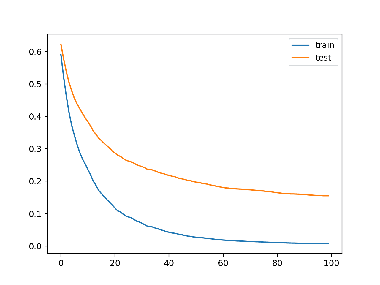
First, the model performance is reported, showing that the model achieved a nomenclature verism of well-nigh 94.5% on the hold-out test set.

The plot shows learning curves for the train and test dataset where the x-axis is the number of iterations of the algorithm (or the number of trees widow to the ensemble) and the y-axis is the logloss of the model. Each line shows the logloss per iteration for a given dataset.

From the learning curves, we can see that the performance of the model on the training dataset (blue line) is largest or has lower loss than the performance of the model on the test dataset (orange line), as we might often expect.

Now that we know how to plot learning curves for XGBoost models, let’s squint at how we might use the curves to modernize model performance.

Tune XGBoost Model Using Learning Curves

We can use the learning curves as a diagnostic tool.

The curves can be interpreted and used as the understructure for suggesting explicit changes to the model configuration that might result in largest performance.

The model and result in the previous section can be used as a baseline and starting point.

Looking at the plot, we can see that both curves are sloping lanugo and suggest that increasingly iterations (adding increasingly trees) may result in a remoter subtract in loss.

Let’s try it out.

We can increase the number of iterations of the algorithm via the “n_estimators” hyperparameter that defaults to 100. Let’s increase it to 500.

The well-constructed example is listed below.

Running the example fits and evaluates the model and plots the learning curves of model performance.

Note: Your results may vary given the stochastic nature of the algorithm or evaluation procedure, or differences in numerical precision. Consider running the example a few times and compare the stereotype outcome.

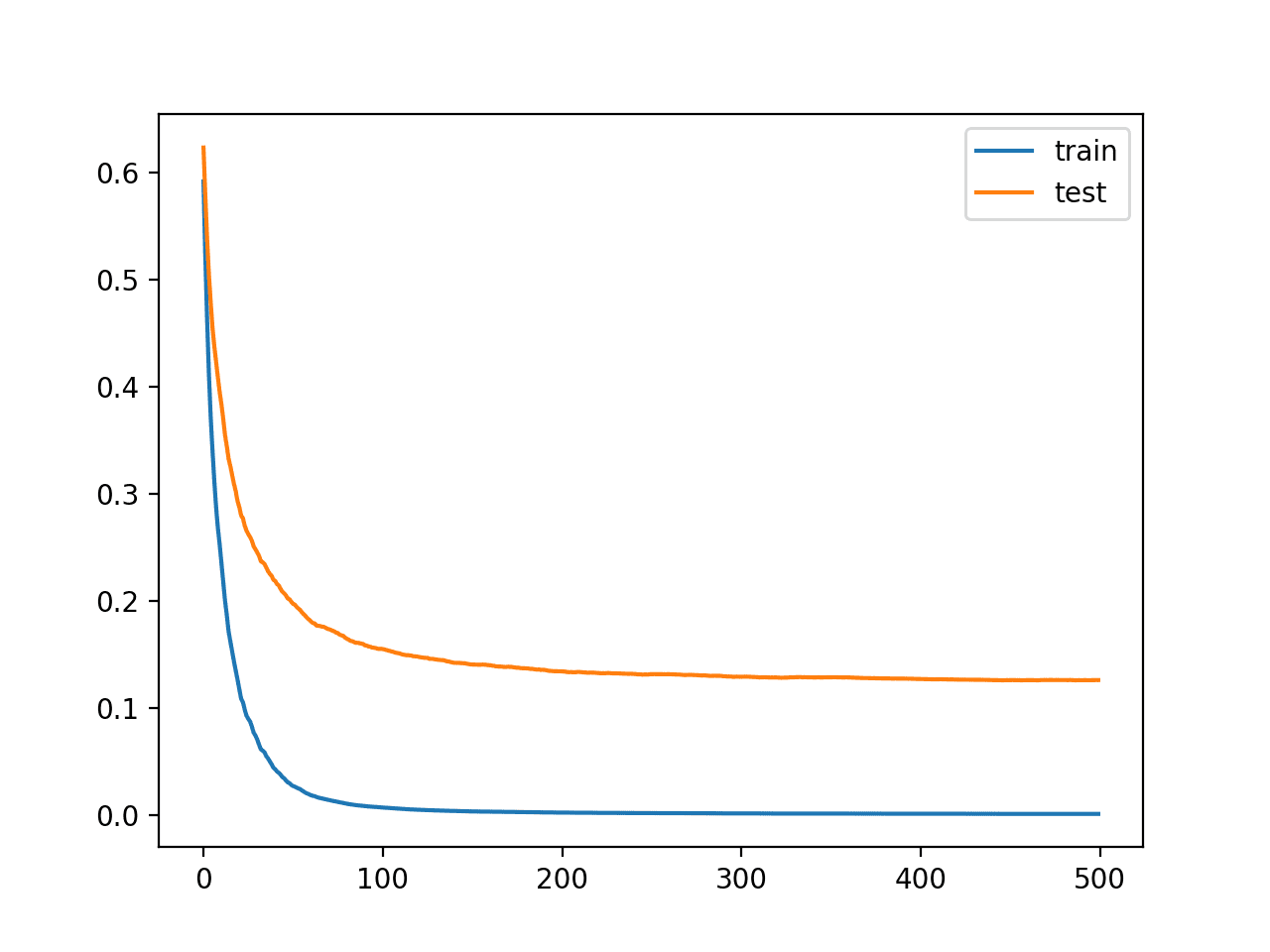
We can see that increasingly iterations have resulted in a lift in verism from well-nigh 94.5% to well-nigh 95.8%.

We can see from the learning curves that indeed the spare iterations of the algorithm caused the curves to protract to waif and then level out without perhaps 150 iterations, where they remain reasonably flat.

The long unappetizing curves may suggest that the algorithm is learning too fast and we may goody from slowing it down.

This can be achieved using the learning rate, which limits the contribution of each tree widow to the ensemble. This can be controlled via the “eta” hyperparameter and defaults to the value of 0.3. We can try a smaller value, such as 0.05.

The well-constructed example is listed below.

Running the example fits and evaluates the model and plots the learning curves of model performance.

Note: Your results may vary given the stochastic nature of the algorithm or evaluation procedure, or differences in numerical precision. Consider running the example a few times and compare the stereotype outcome.

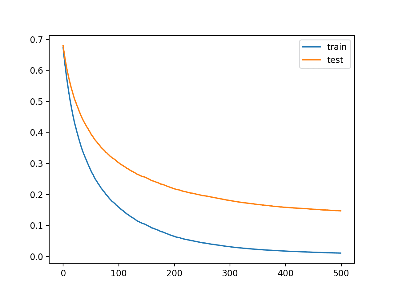
We can see that the smaller learning rate has made the verism worse, dropping from well-nigh 95.8% to well-nigh 95.1%.

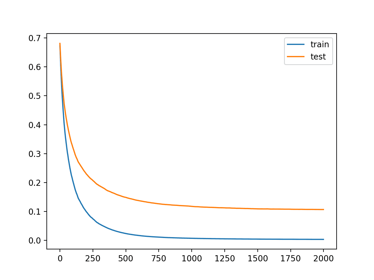
We can see from the learning curves that indeed learning has slowed right down. The curves suggest that we can protract to add increasingly iterations and perhaps unzip largest performance as the curves would have increasingly opportunity to protract to decrease.

Let’s try increasing the number of iterations from 500 to 2,000.

The well-constructed example is listed below.

Running the example fits and evaluates the model and plots the learning curves of model performance.

Note: Your results may vary given the stochastic nature of the algorithm or evaluation procedure, or differences in numerical precision. Consider running the example a few times and compare the stereotype outcome.

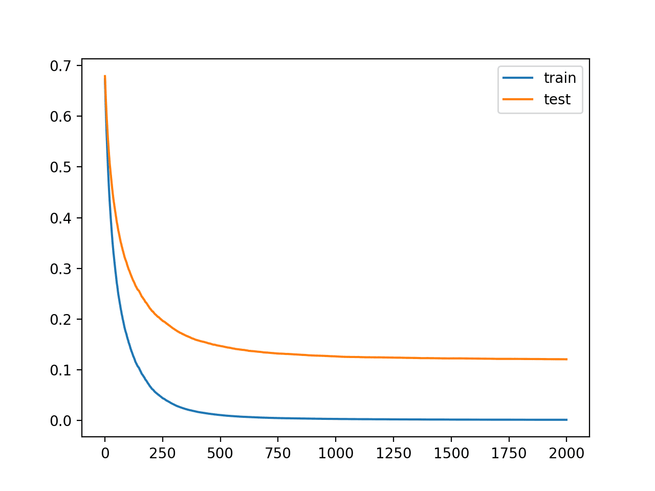
We can see that increasingly iterations have given the algorithm increasingly space to improve, achieving an verism of 96.1%, the weightier so far.

The learning curves then show a stable convergence of the algorithm with a steep subtract and long flattening out.

We could repeat the process of decreasing the learning rate and increasing the number of iterations to see if remoter improvements are possible.

Another tideway to slowing lanugo learning is to add regularization in the form of reducing the number of samples and features (rows and columns) used to construct each tree in the ensemble.

In this case, we will try halving the number of samples and features respectively via the “subsample” and “colsample_bytree” hyperparameters.

The well-constructed example is listed below.

Running the example fits and evaluates the model and plots the learning curves of model performance.

Note: Your results may vary given the stochastic nature of the algorithm or evaluation procedure, or differences in numerical precision. Consider running the example a few times and compare the stereotype outcome.

We can see that the wing of regularization has resulted in a remoter improvement, bumping verism from well-nigh 96.1% to well-nigh 96.6%.

The curves suggest that regularization has  slowed learning and that perhaps increasing the number of iterations may result in remoter improvements.

This process can continue, and I am interested to see what you can come up with.

Further Reading

This section provides increasingly resources on the topic if you are looking to go deeper.

Tutorials

Papers

APIs

Summary

In this tutorial, you discovered how to plot and interpret learning curves for XGBoost models in Python.

Specifically, you learned:

• Learning curves provide a useful diagnostic tool for understanding the training dynamics of supervised learning models like XGBoost.
• How to configure XGBoost to evaluate datasets each iteration and plot the results as learning curves.
• How to interpret and use learning lines plots to modernize XGBoost model performance.

Do you have any questions?
Ask your questions in the comments unelevated and I will do my weightier to answer.