Tweet
Share
Share
Last Updated on November 20, 2021
Convolutional neural networks have their roots in image processing. It was first published
2.9k
By Nick Cotes
Last Updated on November 20, 2021
Convolutional neural networks have their roots in image processing. It was first published in LeNet to recognize the MNIST handwritten digits. However, convolutional neural networks are not limited to handling images.
In this tutorial, we are going to look at an example of using CNN for time series prediction with an application from financial markets. By way of this example, we are going to explore some techniques in using Keras for model training as well.
After completing this tutorial, you will know
What a typical multidimensional financial data series looks like?
How can CNN applied to time series in a classification problem
How to use generators to feed data to train a Keras model
How to provide a custom metric for evaluating a Keras model
Let’s get started
Using CNN for financial time series prediction Photo by Aron Visuals, some rights reserved.
Tutorial overview
This tutorial is divided into 7 parts; they are:
Background of the idea
Preprocessing of data
Data generator
The model
Training, validation, and test
Extensions
Does it work?
Background of the idea
In this tutorial we are following the paper titled “CNNpred: CNN-based stock market prediction using a iverse set of variables” by Ehsan Hoseinzade and Saman Haratizadeh. The data file and sample code from the author are available in github:
The goal of the paper is simple: To predict the next day’s direction of the stock market (i.e., up or down compared to today), hence it is a binary classification problem. However, it is interesting to see how this problem are formulated and solved.
We have seen the examples on using CNN for sequence prediction. If we consider Dow Jones Industrial Average (DJIA) as an example, we may build a CNN with 1D convolution for prediction. This makes sense because a 1D convolution on a time series is roughly computing its moving average or using digital signal processing terms, applying a filter to the time series. It should provide some clues about the trend.
However, when we look at financial time series, it is quite a common sense that some derived signals are useful for predictions too. For example, price and volume together can provide a better clue. Also some other technical indicators such as the moving average of different window size are useful too. If we put all these align together, we will have a table of data, which each time instance has multiple features, and the goal is still to predict the direction of one time series.
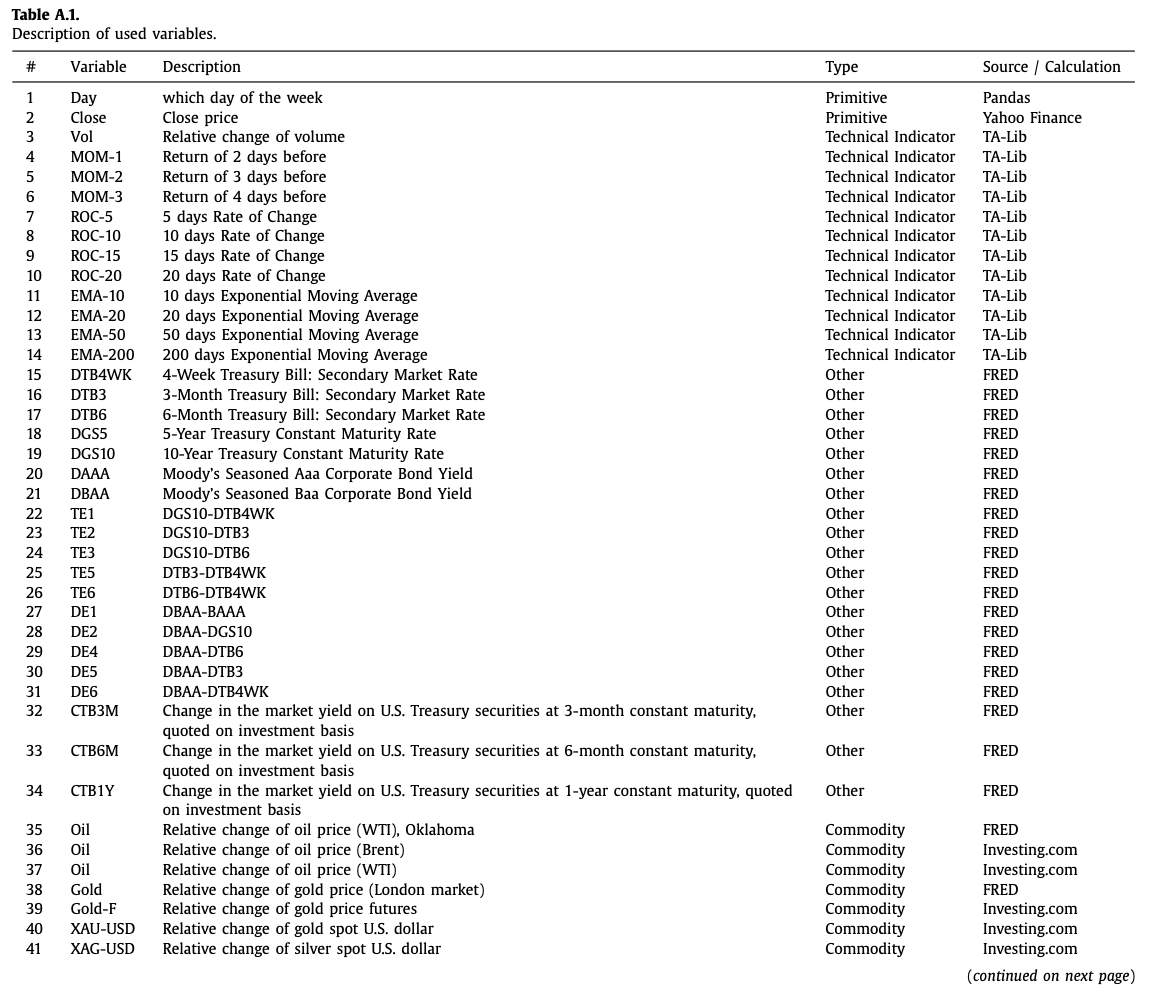
In the CNNpred paper, 82 such features are prepared for the DJIA time series:
Excerpt from the CNNpred paper showing the list of features used.
Unlike LSTM, which there is an explicit concept of time steps applied, we present data as a matrix in CNN models. As shown in the table below, the features across multiple time steps are presented as a 2D array.
Preprocessing of data
In the following, we try to implement the idea of the CNNpred from scratch using Tensorflow’s keras API. While there is a reference implementation from the author in the github link above, we reimplement it differently to illustrate some Keras techniques.
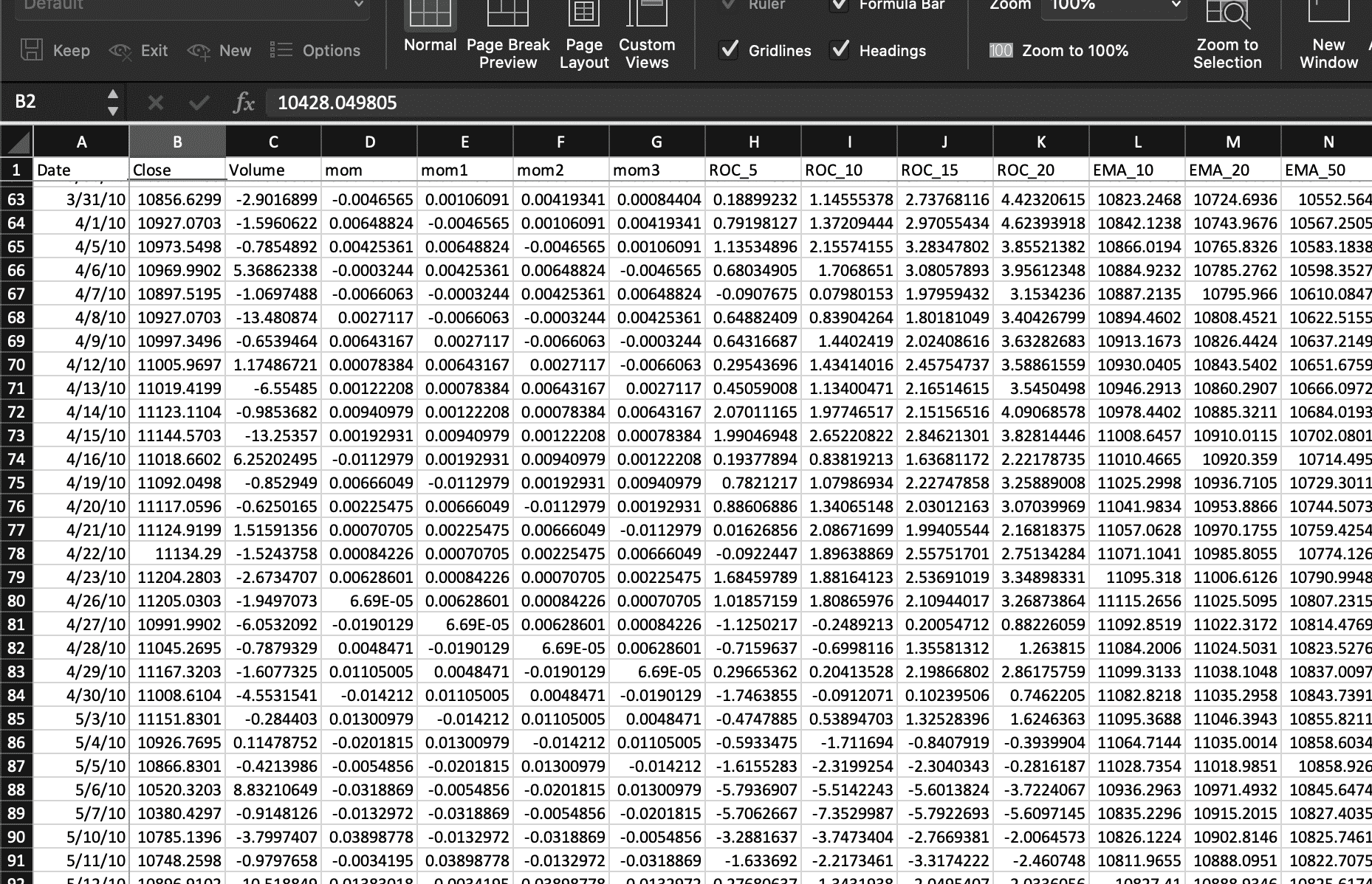
Firstly the data are five CSV files, each for a different market index, under the Dataset directory from github repository above, or we can also get a copy here:
The input data has a date column and a name column to identify the ticker symbol for the market index. We can leave the date column as time index and remove the name column. The rest are all numerical.
As we are going to predict the market direction, we first try to create the classification label. The market direction is defined as the closing index of tomorrow compared to today. If we have read the data into a pandas DataFrame, we can use X["Close"].pct_change() to find the percentage change, which a positive change for the market goes up. So we can shift this to one time step back as our label:
The line of code above is to compute the percentage change of the closing index and align the data with the previous day. Then convert the data into either 1 or 0 for whether the percentage change is positive.
For five data file in the directory, we read each of them as a separate pandas DataFrame and keep them in a Python dictionary:
# Fit the standard scaler using the training dataset
index=X.index[X.index>TRAIN_TEST_CUTOFF]
index=index[:int(len(index)*TRAIN_VALID_RATIO)]
scaler=StandardScaler().fit(X.loc[index,cols])
# Save scale transformed dataframe
X[cols]=scaler.transform(X[cols])
data[name]=X
The result of the above code is a DataFrame for each index, which the classification label is the column “Target” while all other columns are input features. We also normalize the data with a standard scaler.
In time series problems, it is generally reasonable not to split the data into training and test sets randomly, but to set up a cutoff point in which the data before the cutoff is training set while that afterwards is the test set. The scaling above are based on the training set but applied to the entire dataset.
Data generator
We are not going to use all time steps at once, but instead, we use a fixed length of N time steps to predict the market direction at step N+1. In this design, the window of N time steps can start from anywhere. We can just create a large number of DataFrames with large amount of overlaps with one another. To save memory, we are going to build a data generator for training and validation, as follows:
Generator is a special function in Python that does not return a value but to yield in iterations, such that a sequence of data are produced from it. For a generator to be used in Keras training, it is expected to yield a batch of input data and target. This generator supposed to run indefinitely. Hence the generator function above is created with an infinite loop starts with while True.
In each iteration, it randomly pick one DataFrame from the Python dictionary, then within the range of time steps of the training set (i.e., the beginning portion), we start from a random point and take N time steps using the pandas iloc[start:end] syntax to create a input under the variable frame. This DataFrame will be a 2D array. The target label is that of the last time step. The input data and the label are then appended to the list batch. Until we accumulated for one batch’s size, we dispatch it from the generator.
The last four lines at the code snippet above is to dispatch a batch for training or validation. We collect the list of input data (each a 2D array) as well as a list of target label into variables X and y, then convert them into numpy array so it can work with our Keras model. We need to add one more dimension to the numpy array X using np.expand_dims() because of the design of the network model, as explained below.
The Model
The 2D CNN model presented in the original paper accepts an input tensor of shape $Ntimes m times 1$ for N the number of time steps and m the number of features in each time step. The paper assumes $N=60$ and $m=82$.
The model comprises of three convolutional layers, as described as follows:
The first convolutional layer has 8 units, and is applied across all features in each time step. It is followed by a second convolutional layer to consider three consecutive days at once, for it is a common belief that three days can make a trend in the stock market. It is then applied to a max pooling layer and another convolutional layer before it is flattened into a one-dimensional array and applied to a fully-connected layer with sigmoid activation for binary classification.
Training, validation, and test
That’s it for the model. The paper used MAE as the loss metric and also monitor for accuracy and F1 score to determine the quality of the model. We should point out that F1 score depends on precision and recall ratios, which are both considering the positive classification. The paper, however, consider the average of the F1 from positive and negative classification. Explicitly, it is the F1-macro metric: $$ F_1 = frac{1}{2}left( frac{2cdot frac{TP}{TP+FP} cdot frac{TP}{TP+FN}}{frac{TP}{TP+FP} + frac{TP}{TP+FN}} + frac{2cdot frac{TN}{TN+FN} cdot frac{TN}{TN+FP}}{frac{TN}{TN+FN} + frac{TN}{TN+FP}} right) $$ The fraction $frac{TP}{TP+FP}$ is the precision with TP and FP the number of true positive and false positive. Similarly $frac{TP}{TP+FN}$ is the recall. The first term in the big parenthesis above is the normal F1 metric that considered positive classifications. And the second term is the reverse, which considered the negative classifications.
While this metric is available in scikit-learn as sklearn.metrics.f1_score() there is no equivalent in Keras. Hence we would create our own by borrowing code from this stackexchange question:
The training process can take hours to complete. Hence we want to save the model in the middle of the training so that we may interrupt and resume it. We can make use of checkpoint features in Keras:
We set up a filename template checkpoint_path and ask Keras to fill in the epoch number as well as validation F1 score into the filename. We save it by monitoring the validation’s F1 metric, and this metric is supposed to increase when the model gets better. Hence we pass in the mode="max" to it.
It should now be trivial to train our model, as follows:
Two points to note in the above snippets. We supplied "acc" as the accuracy as well as the function f1macro defined above as the metrics parameter to the compile() function. Hence these two metrics will be monitored during training. Because the function is named f1macro, we refer to this metric in the checkpoint’s monitor parameter as val_f1macro.
Separately, in the fit() function, we provided the input data through the datagen() generator as defined above. Calling this function will produce a generator, which during the training loop, batches are fetched from it one after another. Similarly, validation data are also provided by the generator.
Because the nature of a generator is to dispatch data indefinitely. We need to tell the training process on how to define a epoch. Recall that in Keras terms, a batch is one iteration of doing gradient descent update. An epoch is supposed to be one cycle through all data in the dataset. At the end of an epoch is the time to run validation. It is also the opportunity for running the checkpoint we defined above. As Keras has no way to infer the size of the dataset from a generator, we need to tell how many batch it should process in one epoch using the steps_per_epoch parameter. Similarly, it is the validation_steps parameter to tell how many batch are used in each validation step. The validation does not affect the training, but it will report to us the metrics we are interested. Below is a screenshot of what we will see in the middle of training, which we will see that the metric for training set are updated on each batch but that for validation set is provided only at the end of epoch:
After the model finished training, we can test it with unseen data, i.e., the test set. Instead of generating the test set randomly, we create it from the dataset in a deterministic way:
The structure of the function testgen() is resembling that of datagen() we defined above. Except in datagen() the output data’s first dimension is the number of samples in a batch but in testgen() is the the entire test samples.
Using the model for prediction will produce a floating point between 0 and 1 as we are using the sigmoid activation function. We will convert this into 0 or 1 by using the threshold at 0.5. Then we use the functions from scikit-learn to compute the accuracy, mean absolute error and F1 score (which accuracy is just one minus the MAE).
Tying all these together, the complete code is as follows:
1
2
3
4
5
6
7
8
9
10
11
12
13
14
15
16
17
18
19
20
21
22
23
24
25
26
27
28
29
30
31
32
33
34
35
36
37
38
39
40
41
42
43
44
45
46
47
48
49
50
51
52
53
54
55
56
57
58
59
60
61
62
63
64
65
66
67
68
69
70
71
72
73
74
75
76
77
78
79
80
81
82
83
84
85
86
87
88
89
90
91
92
93
94
95
96
97
98
99
100
101
102
103
104
105
106
107
108
109
110
111
112
113
114
115
116
117
118
119
120
121
122
123
124
125
126
127
128
129
130
131
132
133
134
135
136
137
138
139
140
141
142
143
144
145
146
147
148
149
150
151
152
153
154
155
156
157
158
import os
import random
import numpy asnp
import pandas aspd
import tensorflow astf
from tensorflow.keras import backend asK
from tensorflow.keras.layers import Dense,Dropout,Flatten,Conv2D,MaxPool2D,Input
from tensorflow.keras.models import Sequential,load_model
from tensorflow.keras.callbacks import ModelCheckpoint
from sklearn.preprocessing import StandardScaler
from sklearn.metrics import accuracy_score,f1_score,mean_absolute_error
The original paper called the above model “2D-CNNpred” and there is a version called “3D-CNNpred”. The idea is not only consider the many features of one stock market index but cross compare with many market indices to help prediction on one index. Refer to the table of features and time steps above, the data for one market index is presented as 2D array. If we stack up multiple such data from different indices, we constructed a 3D array. While the target label is the same, but allowing us to look at a different market may provide some additional information to help prediction.
Because the shape of the data changed, the convolutional network also defined slightly different, and the data generators need some modification accordingly as well. Below is the complete code of the 3D version, which the change from the previous 2d version should be self-explanatory:
1
2
3
4
5
6
7
8
9
10
11
12
13
14
15
16
17
18
19
20
21
22
23
24
25
26
27
28
29
30
31
32
33
34
35
36
37
38
39
40
41
42
43
44
45
46
47
48
49
50
51
52
53
54
55
56
57
58
59
60
61
62
63
64
65
66
67
68
69
70
71
72
73
74
75
76
77
78
79
80
81
82
83
84
85
86
87
88
89
90
91
92
93
94
95
96
97
98
99
100
101
102
103
104
105
106
107
108
109
110
111
112
113
114
115
116
117
118
119
120
121
122
123
124
125
126
127
128
129
130
131
132
133
134
135
136
137
138
139
140
141
142
143
144
145
146
147
148
149
150
151
152
153
154
155
156
157
158
159
160
161
162
163
164
165
166
167
168
169
170
171
172
173
174
175
176
177
import os
import random
import numpy asnp
import pandas aspd
import tensorflow astf
from tensorflow.keras import backend asK
from tensorflow.keras.layers import Dense,Dropout,Flatten,Conv2D,MaxPool2D,Input
from tensorflow.keras.models import Sequential,load_model
from tensorflow.keras.callbacks import ModelCheckpoint
from sklearn.preprocessing import StandardScaler
from sklearn.metrics import accuracy_score,f1_score,mean_absolute_error
While the model above is for next-step prediction, it does not stop you from making prediction for k steps ahead if you replace the target label to a different calculation. This may be an exercise for you.
Does it work?
As in all prediction projects in the financial market, it is always unrealistic to expect a high accuracy. The training parameter in the code above can produce slightly more than 50% accuracy in the testing set. While the number of epochs and batch size are deliberately set smaller to save time, there should not be much room for improvement.
In the original paper, it is reported that the 3D-CNNpred performed better than 2D-CNNpred but only attaining the F1 score of less than 0.6. This is already doing better than three baseline models mentioned in the paper. It may be of some use, but not a magic that can help you make money quick.
From machine learning technique perspective, here we classify a panel of data into whether the market direction is up or down the next day. Hence while the data is not an image, it resembles one since both are presented in the form of a 2D array. The technique of convolutional layers can therefore applied, but we may use a different filter size to match the intuition we usually have for financial time series.
Further readings
The original paper is available at:
If you are new to finance application and want to build the connection between machine learning techniques and finance, you may find this book useful:
On the similar topic, we have a previous post on using CNN for time series, but using 1D convolutional layers;
You may also find the following documentation helpful to explain some syntax we used above:
Summary
In this tutorial, you discovered how a CNN model can be built for prediction in financial time series.
Specifically, you learned:
How to create 2D convolutional layers to process the time series
How to present the time series data in a multidimensional array so that the convolutional layers can be applied
What is a data generator for Keras model training and how to use it
How to monitor the performance of model training with a custom metric