Real Python: Combining Data in Pandas With merge(), .join(), and concat()
The Series and DataFrame objects in pandas are powerful tools for exploring and analyzing data. Part of their power comes from a multifaceted approach to combining separate datasets. With pandas,
8.2k
By Amol Rathi
The Series and DataFrame objects in pandas are powerful tools for exploring and analyzing data. Part of their power comes from a multifaceted approach to combining separate datasets. With pandas, you can merge, join, and concatenate your datasets, allowing you to unify and better understand your data as you analyze it.
In this tutorial, you’ll learn how and when to combine your data in pandas with:
merge() for combining data on common columns or indices
.join() for combining data on a key column or an index
concat() for combining DataFrames across rows or columns
If you have some experience using DataFrame and Series objects in pandas and you’re ready to learn how to combine them, then this tutorial will help you do exactly that. If you’re feeling a bit rusty, then you can watch a quick refresher on DataFrames before proceeding.
You can follow along with the examples in this tutorial using the interactive Jupyter Notebook and data files available at the link below:
Note: The techniques that you’ll learn about below will generally work for both DataFrame and Series objects. But for simplicity and concision, the examples will use the term dataset to refer to objects that can be either DataFrames or Series.
pandas merge(): Combining Data on Common Columns or Indices
The first technique that you’ll learn is merge(). You can use merge() anytime you want functionality similar to a database’s join operations. It’s the most flexible of the three operations that you’ll learn.
When you want to combine data objects based on one or more keys, similar to what you’d do in a relational database, merge() is the tool you need. More specifically, merge() is most useful when you want to combine rows that share data.
You can achieve both many-to-one and many-to-many joins with merge(). In a many-to-one join, one of your datasets will have many rows in the merge column that repeat the same values. For example, the values could be 1, 1, 3, 5, and 5. At the same time, the merge column in the other dataset won’t have repeated values. Take 1, 3, and 5 as an example.
As you might have guessed, in a many-to-many join, both of your merge columns will have repeated values. These merges are more complex and result in the Cartesian product of the joined rows.
This means that, after the merge, you’ll have every combination of rows that share the same value in the key column. You’ll see this in action in the examples below.
What makes merge() so flexible is the sheer number of options for defining the behavior of your merge. While the list can seem daunting, with practice you’ll be able to expertly merge datasets of all kinds.
When you use merge(), you’ll provide two required arguments:
The left DataFrame
The right DataFrame
After that, you can provide a number of optional arguments to define how your datasets are merged:
how defines what kind of merge to make. It defaults to 'inner', but other possible options include 'outer', 'left', and 'right'.
on tells merge() which columns or indices, also called key columns or key indices, you want to join on. This is optional. If it isn’t specified, and left_index and right_index (covered below) are False, then columns from the two DataFrames that share names will be used as join keys. If you use on, then the column or index that you specify must be present in both objects.
left_on and right_on specify a column or index that’s present only in the left or right object that you’re merging. Both default to None.
left_index and right_index both default to False, but if you want to use the index of the left or right object to be merged, then you can set the relevant argument to True.
suffixes is a tuple of strings to append to identical column names that aren’t merge keys. This allows you to keep track of the origins of columns with the same name.
These are some of the most important parameters to pass to merge(). For the full list, see the pandas documentation.
Note: In this tutorial, you’ll see that examples always use on to specify which column(s) to join on. This is the safest way to merge your data because you and anyone reading your code will know exactly what to expect when calling merge(). If you don’t specify the merge column(s) with on, then pandas will use any columns with the same name as the merge keys.
How to Use merge()
Before getting into the details of how to use merge(), you should first understand the various forms of joins:
inner
outer
left
right
Note: Even though you’re learning about merging, you’ll see inner, outer, left, and right also referred to as join operations. For this tutorial, you can consider the terms merge and join equivalent.
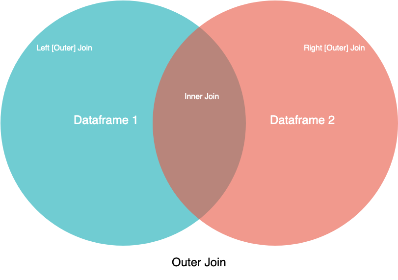
You’ll learn about these different joins in detail below, but first take a look at this visual representation of them:
Visual Representation of Join Types
In this image, the two circles are your two datasets, and the labels point to which part or parts of the datasets you can expect to see. While this diagram doesn’t cover all the nuance, it can be a handy guide for visual learners.
If you have an SQL background, then you may recognize the merge operation names from the JOIN syntax. Except for inner, all of these techniques are types of outer joins. With outer joins, you’ll merge your data based on all the keys in the left object, the right object, or both. For keys that only exist in one object, unmatched columns in the other object will be filled in with NaN, which stands for Not a Number.
You can also see a visual explanation of the various joins in an SQL context on Coding Horror. Now take a look at the different joins in action.
Examples
Many pandas tutorials provide very simple DataFrames to illustrate the concepts that they are trying to explain. This approach can be confusing since you can’t relate the data to anything concrete. So, for this tutorial, you’ll use two real-world datasets as the DataFrames to be merged:
Climate normals for California (temperatures)
Climate normals for California (precipitation)
You can explore these datasets and follow along with the examples below using the interactive Jupyter Notebook and climate data CSVs:
If you’d like to learn how to use Jupyter Notebooks, then check out Jupyter Notebook: An Introduction.
These two datasets are from the National Oceanic and Atmospheric Administration (NOAA) and were derived from the NOAA public data repository. First, load the datasets into separate DataFrames:
In the code above, you used pandas’ read_csv() to conveniently load your source CSV files into DataFrame objects. You can then look at the headers and first few rows of the loaded DataFrames with .head():
>>>
>>> climate_temp.head() STATION STATION_NAME ... DLY-HTDD-BASE60 DLY-HTDD-NORMAL0 GHCND:USC00049099 TWENTYNINE PALMS CA US ... 10 151 GHCND:USC00049099 TWENTYNINE PALMS CA US ... 10 152 GHCND:USC00049099 TWENTYNINE PALMS CA US ... 10 153 GHCND:USC00049099 TWENTYNINE PALMS CA US ... 10 154 GHCND:USC00049099 TWENTYNINE PALMS CA US ... 10 15>>> climate_precip.head() STATION ... DLY-SNOW-PCTALL-GE050TI0 GHCND:USC00049099 ... -99991 GHCND:USC00049099 ... -99992 GHCND:USC00049099 ... -99993 GHCND:USC00049099 ... 04 GHCND:USC00049099 ... 0
Here, you used .head() to get the first five rows of each DataFrame. Make sure to try this on your own, either with the interactive Jupyter Notebook or in your console, so that you can explore the data in greater depth.
Next, take a quick look at the dimensions of the two DataFrames:
Note that .shape is a property of DataFrame objects that tells you the dimensions of the DataFrame. For climate_temp, the output of .shape says that the DataFrame has 127,020 rows and 21 columns.
Inner Join
In this example, you’ll use merge() with its default arguments, which will result in an inner join. Remember that in an inner join, you’ll lose rows that don’t have a match in the other DataFrame’s key column.
With the two datasets loaded into DataFrame objects, you’ll select a small slice of the precipitation dataset and then use a plain merge() call to do an inner join. This will result in a smaller, more focused dataset:
Here you’ve created a new DataFrame called precip_one_station from the climate_precip DataFrame, selecting only rows in which the STATION field is "GHCND:USC00045721".
If you check the shape attribute, then you’ll see that it has 365 rows. When you do the merge, how many rows do you think you’ll get in the merged DataFrame? Remember that you’ll be doing an inner join:
>>>
>>> inner_merged=pd.merge(precip_one_station,climate_temp)>>> inner_merged.head() STATION STATION_NAME ... DLY-HTDD-BASE60 DLY-HTDD-NORMAL0 GHCND:USC00045721 MITCHELL CAVERNS CA US ... 14 191 GHCND:USC00045721 MITCHELL CAVERNS CA US ... 14 192 GHCND:USC00045721 MITCHELL CAVERNS CA US ... 14 193 GHCND:USC00045721 MITCHELL CAVERNS CA US ... 14 194 GHCND:USC00045721 MITCHELL CAVERNS CA US ... 14 19>>> inner_merged.shape(365, 47)
If you guessed 365 rows, then you were correct! This is because merge() defaults to an inner join, and an inner join will discard only those rows that don’t match. Because all of your rows had a match, none were lost. You should also notice that there are many more columns now: 47 to be exact.
With merge(), you also have control over which column(s) to join on. Let’s say that you want to merge both entire datasets, but only on Station and Date since the combination of the two will yield a unique value for each row. To do so, you can use the on parameter:
You can specify a single key column with a string or multiple key columns with a list. This results in a DataFrame with 123,005 rows and 48 columns.
Why 48 columns instead of 47? Because you specified the key columns to join on, pandas doesn’t try to merge all mergeable columns. This can result in “duplicate” column names, which may or may not have different values.
“Duplicate” is in quotation marks because the column names will not be an exact match. By default, they are appended with _x and _y. You can also use the suffixes parameter to control what’s appended to the column names.
To prevent surprises, all the following examples will use the on parameter to specify the column or columns on which to join.
Outer Join
Here, you’ll specify an outer join with the how parameter. Remember from the diagrams above that in an outer join—also known as a full outer join—all rows from both DataFrames will be present in the new DataFrame.
If a row doesn’t have a match in the other DataFrame based on the key column(s), then you won’t lose the row like you would with an inner join. Instead, the row will be in the merged DataFrame, with NaN values filled in where appropriate.
If you remember from when you checked the .shape attribute of climate_temp, then you’ll see that the number of rows in outer_merged is the same. With an outer join, you can expect to have the same number of rows as the larger DataFrame. That’s because no rows are lost in an outer join, even when they don’t have a match in the other DataFrame.
Left Join
In this example, you’ll specify a left join—also known as a left outer join—with the how parameter. Using a left outer join will leave your new merged DataFrame with all rows from the left DataFrame, while discarding rows from the right DataFrame that don’t have a match in the key column of the left DataFrame.
You can think of this as a half-outer, half-inner merge. The example below shows you this in action:
left_merged has 127,020 rows, matching the number of rows in the left DataFrame, climate_temp. To prove that this only holds for the left DataFrame, run the same code, but change the position of precip_one_station and climate_temp:
This results in a DataFrame with 365 rows, matching the number of rows in precip_one_station.
Right Join
The right join, or right outer join, is the mirror-image version of the left join. With this join, all rows from the right DataFrame will be retained, while rows in the left DataFrame without a match in the key column of the right DataFrame will be discarded.
To demonstrate how right and left joins are mirror images of each other, in the example below you’ll recreate the left_merged DataFrame from above, only this time using a right join:
Here, you simply flipped the positions of the input DataFrames and specified a right join. When you inspect right_merged, you might notice that it’s not exactly the same as left_merged. The only difference between the two is the order of the columns: the first input’s columns will always be the first in the newly formed DataFrame.
merge() is the most complex of the pandas data combination tools. It’s also the foundation on which the other tools are built. Its complexity is its greatest strength, allowing you to combine datasets in every which way and to generate new insights into your data.
On the other hand, this complexity makes merge() difficult to use without an intuitive grasp of set theory and database operations. In this section, you’ve learned about the various data merging techniques, as well as many-to-one and many-to-many merges, which ultimately come from set theory. For more information on set theory, check out Sets in Python.
Now, you’ll look at .join(), a simplified version of merge().
pandas .join(): Combining Data on a Column or Index
While merge() is a module function, .join() is an instance method that lives on your DataFrame. This enables you to specify only one DataFrame, which will join the DataFrame you call .join() on.
Under the hood, .join() uses merge(), but it provides a more efficient way to join DataFrames than a fully specified merge() call. Before diving into the options available to you, take a look at this short example:
With the indices visible, you can see a left join happening here, with precip_one_station being the left DataFrame. You might notice that this example provides the parameters lsuffix and rsuffix. Because .join() joins on indices and doesn’t directly merge DataFrames, all columns—even those with matching names—are retained in the resulting DataFrame.
Now flip the previous example around and instead call .join() on the larger DataFrame:
Notice that the DataFrame is larger, but data that doesn’t exist in the smaller DataFrame, precip_one_station, is filled in with NaN values.
How to Use .join()
By default, .join() will attempt to do a left join on indices. If you want to join on columns like you would with merge(), then you’ll need to set the columns as indices.
Like merge(), .join() has a few parameters that give you more flexibility in your joins. However, with .join(), the list of parameters is relatively short:
other is the only required parameter. It defines the other DataFrame to join. You can also specify a list of DataFrames here, allowing you to combine a number of datasets in a single .join() call.
on specifies an optional column or index name for the left DataFrame (climate_temp in the previous example) to join the other DataFrame’s index. If it’s set to None, which is the default, then you’ll get an index-on-index join.
how has the same options as how from merge(). The difference is that it’s index-based unless you also specify columns with on.
lsuffix and rsuffix are similar to suffixes in merge(). They specify a suffix to add to any overlapping columns but have no effect when passing a list of other DataFrames.
sort can be enabled to sort the resulting DataFrame by the join key.
Examples
In this section, you’ll see examples showing a few different use cases for .join(). Some will be simplifications of merge() calls. Others will be features that set .join() apart from the more verbose merge() calls.
Since you already saw a short .join() call, in this first example you’ll attempt to recreate a merge() call with .join(). What will this require? Take a second to think about a possible solution, and then look at the proposed solution below:
Because .join() works on indices, if you want to recreate merge() from before, then you must set indices on the join columns that you specify. In this example, you used .set_index() to set your indices to the key columns within the join. Note that .join() does a left join by default so you need to explictly use how to do an inner join.
With this, the connection between merge() and .join() should be clearer.
Below you’ll see a .join() call that’s almost bare. Because there are overlapping columns, you’ll need to specify a suffix with lsuffix, rsuffix, or both, but this example will demonstrate the more typical behavior of .join():
This example should be reminiscent of what you saw in the introduction to .join() earlier. The call is the same, resulting in a left join that produces a DataFrame with the same number of rows as climate_temp.
In this section, you’ve learned about .join() and its parameters and uses. You’ve also learned about how .join() works under the hood, and you’ve recreated a merge() call with .join() to better understand the connection between the two techniques.
pandas concat(): Combining Data Across Rows or Columns
Concatenation is a bit different from the merging techniques that you saw above. With merging, you can expect the resulting dataset to have rows from the parent datasets mixed in together, often based on some commonality. Depending on the type of merge, you might also lose rows that don’t have matches in the other dataset.
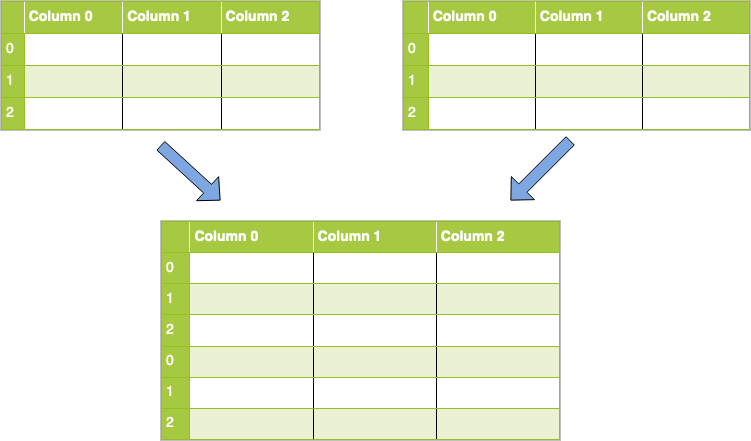
With concatenation, your datasets are just stitched together along an axis — either the row axis or column axis. Visually, a concatenation with no parameters along rows would look like this:
To implement this in code, you’ll use concat() and pass it a list of DataFrames that you want to concatenate. Code for this task would look like this:
concatenated=pandas.concat([df1,df2])
Note: This example assumes that your column names are the same. If your column names are different while concatenating along rows (axis 0), then by default the columns will also be added, and NaN values will be filled in as applicable.
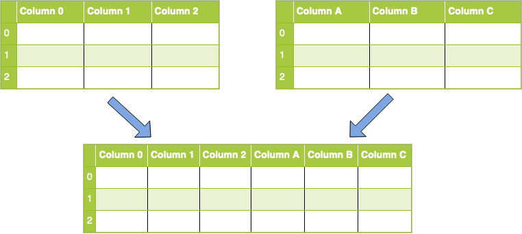
What if you wanted to perform a concatenation along columns instead? First, take a look at a visual representation of this operation:
To accomplish this, you’ll use a concat() call like you did above, but you’ll also need to pass the axis parameter with a value of 1 or "columns":
Note: This example assumes that your indices are the same between datasets. If they’re different while concatenating along columns (axis 1), then by default the extra indices (rows) will also be added, and NaN values will be filled in as applicable.
You’ll learn more about the parameters for concat() in the section below.
How to Use concat()
As you can see, concatenation is a simpler way to combine datasets. It’s often used to form a single, larger set to do additional operations on.
Note: When you call concat(), a copy of all the data that you’re concatenating is made. You should be careful with multiple concat() calls, as the many copies that are made may negatively affect performance. Alternatively, you can set the optional copy parameter to False
When you concatenate datasets, you can specify the axis along which you’ll concatenate. But what happens with the other axis?
Nothing. By default, a concatenation results in a set union, where all data is preserved. You’ve seen this with merge() and .join() as an outer join, and you can specify this with the join parameter.
If you use this parameter, then the default is outer, but you also have the inner option, which will perform an inner join, or set intersection.
As with the other inner joins you saw earlier, some data loss can occur when you do an inner join with concat(). Only where the axis labels match will you preserve rows or columns.
Note: Remember, the join parameter only specifies how to handle the axes that you’re not concatenating along.
Since you learned about the join parameter, here are some of the other parameters that concat() takes:
objs takes any sequence—typically a list—of Series or DataFrame objects to be concatenated. You can also provide a dictionary. In this case, the keys will be used to construct a hierarchical index.
axis represents the axis that you’ll concatenate along. The default value is 0, which concatenates along the index, or row axis. Alternatively, a value of 1 will concatenate vertically, along columns. You can also use the string values "index" or "columns".
join is similar to the how parameter in the other techniques, but it only accepts the values inner or outer. The default value is outer, which preserves data, while inner would eliminate data that doesn’t have a match in the other dataset.
ignore_index takes a Boolean True or False value. It defaults to False. If True, then the new combined dataset won’t preserve the original index values in the axis specified in the axis parameter. This lets you have entirely new index values.
keys allows you to construct a hierarchical index. One common use case is to have a new index while preserving the original indices so that you can tell which rows, for example, come from which original dataset.
copy specifies whether you want to copy the source data. The default value is True. If the value is set to False, then pandas won’t make copies of the source data.
This list isn’t exhaustive. You can find the complete, up-to-date list of parameters in the pandas documentation.
Examples
First, you’ll do a basic concatenation along the default axis using the DataFrames that you’ve been playing with throughout this tutorial:
This one is very simple by design. Here, you created a DataFrame that is a double of a small DataFrame that was made earlier. One thing to notice is that the indices repeat. If you want a fresh, 0-based index, then you can use the ignore_index parameter:
As noted before, if you concatenate along axis 0 (rows) but have labels in axis 1 (columns) that don’t match, then those columns will be added and filled in with NaN values. This results in an outer join:
With these two DataFrames, since you’re just concatenating along rows, very few columns have the same name. That means you’ll see a lot of columns with NaN values.
To instead drop columns that have any missing data, use the join parameter with the value "inner" to do an inner join:
Now you have only the rows that have data for all columns in both DataFrames. It’s no coincidence that the number of rows corresponds with that of the smaller DataFrame.
Another useful trick for concatenation is using the keys parameter to create hierarchical axis labels. This is useful if you want to preserve the indices or column names of the original datasets but also want to add new ones:
If you check on the original DataFrames, then you can verify whether the higher-level axis labels temp and precip were added to the appropriate rows.
Conclusion
You’ve now learned the three most important techniques for combining data in pandas:
merge() for combining data on common columns or indices
.join() for combining data on a key column or an index
concat() for combining DataFrames across rows or columns
In addition to learning how to use these techniques, you also learned about set logic by experimenting with the different ways to join your datasets. Additionally, you learned about the most common parameters to each of the above techniques, and what arguments you can pass to customize their output.
You saw these techniques in action on a real dataset obtained from the NOAA, which showed you not only how to combine your data but also the benefits of doing so with pandas’ built-in techniques. If you haven’t downloaded the project files yet, you can get them here:
Did you learn something new? Figure out a creative way to solve a problem by combining complex datasets? Let us know in the comments below!