Two-Dimensional (2D) Test Functions for Function Optimization
Tweet
Share
Share
Function optimization is a field of study that seeks an input to a function that results in the
9k
By Nick Cotes
Function optimization is a field of study that seeks an input to a function that results in the maximum or minimum output of the function.
There are a large number of optimization algorithms and it is important to study and develop intuitions for optimization algorithms on simple and easy-to-visualize test functions.
Two-dimensional functions take two input values (x and y) and output a each evaluation of the input. They are among the simplest types of test functions to use when studying function optimization. The goody of two-dimensional functions is that they can be visualized as a silhouette plot or surface plot that shows the topography of the problem domain with the optima and samples of the domain marked with points.
In this tutorial, you will discover standard two-dimensional functions you can use when studying function optimization.
Let’s get started.
Two-Dimensional (2D) Test Functions for Function Optimization Photo by DomWphoto, some rights reserved.
Tutorial Overview
A two-dimensional function is a function that takes two input variables and computes the objective value.
We can think of the two input variables as two axes on a graph, x and y. Each input to the function is a each point on the graph and the outcome of the function can be taken as the height on the graph.
This allows the function to be conceptualized as a surface and we can typify the function based on the structure of the surface. For example, hills for input points that result in large relative outcomes of the objective function and valleys for input points that result in small relative outcomes of the objective function.
A surface may have one major full-length or global optima, or it may have many with lots of places for an optimization to get stuck. The surface may be smooth, noisy, convex, and all manner of other properties that we may superintendency well-nigh when testing optimization algorithms.
There are many variegated types of simple two-dimensional test functions we could use.
Nevertheless, there are standard test functions that are wontedly used in the field of function optimization. There are moreover explicit properties of test functions that we may wish to select when testing variegated algorithms.
We will explore a small number of simple two-dimensional test functions in this tutorial and organize them by their properties with two variegated groups; they are:
Unimodal Functions
Unimodal Function 1
Unimodal Function 2
Unimodal Function 3
Multimodal Functions
Multimodal Function 1
Multimodal Function 2
Multimodal Function 3
Each function will be presented using Python lawmaking with a function implementation of the target objective function and a sampling of the function that is shown as a surface plot.
All functions are presented as a minimization function, e.g. find the input that results in the minimum (smallest value) output of the function. Any maximizing function can be made a minimization function by subtracting a negative sign to all output. Similarly, any minimizing function can be made maximizing in the same way.
I did not invent these functions; they are taken from the literature. See the remoter reading section for references.
You can then segregate and copy-paste the lawmaking one or increasingly functions to use in your own project to study or compare the policies of optimization algorithms.
Unimodal Functions
Unimodal ways that the function has a each global optima.
A unimodal function may or may not be convex. A convex function is a function where a line can be drawn between any two points in the domain and the line remains in the domain. For a two-dimensional function shown as a silhouette or surface plot, this ways the function has a trencher shape and the line between two remains whilom or in the bowl.
Let’s squint at a few examples of unimodal functions.
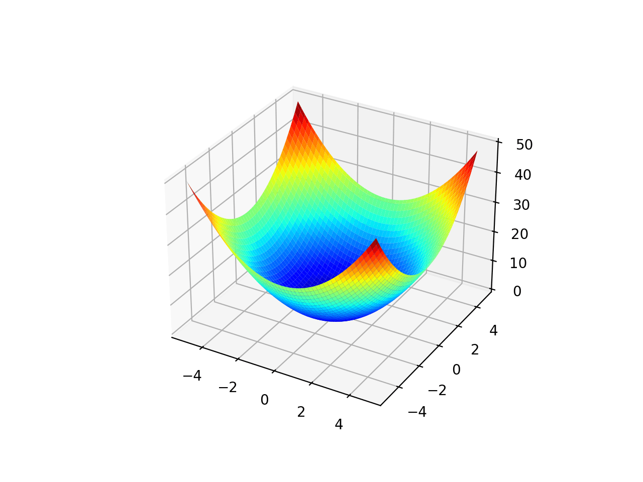
Unimodal Function 1
The range is regional to -5.0 and 5.0 and one global optimal at [0.0, 0.0].
1
2
3
4
5
6
7
8
9
10
11
12
13
14
15
16
17
18
19
20
21
22
23
24
25
# unimodal test function
from numpy import arange
from numpy import meshgrid
from matplotlib import pyplot
from mpl_toolkits.mplot3d import Axes3D
# objective function
def objective(x,y):
returnx**2.0y**2.0
# pinpoint range for input
r_min,r_max=-5.0,5.0
# sample input range uniformly at 0.1 increments
xaxis=arange(r_min,r_max,0.1)
yaxis=arange(r_min,r_max,0.1)
# create a mesh from the axis
x,y=meshgrid(xaxis,yaxis)
# compute targets
results=objective(x,y)
# create a surface plot with the jet verisimilitude scheme
figure=pyplot.figure()
axis=figure.gca(projection='3d')
axis.plot_surface(x,y,results,cmap='jet')
# show the plot
pyplot.show()
Running the example creates a surface plot of the function.
Surface Plot of Unimodal Optimization Function 1
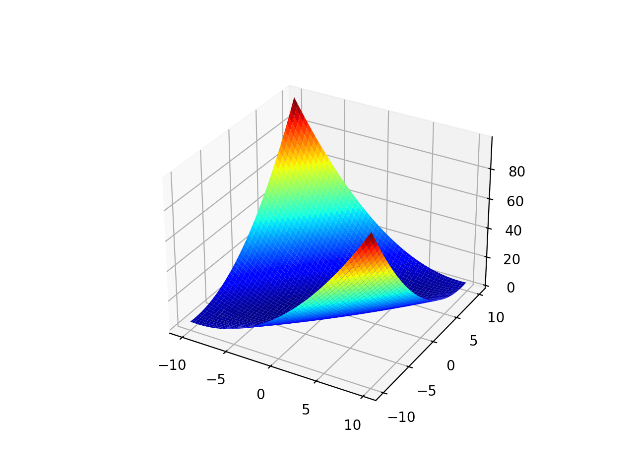
Unimodal Function 2
The range is regional to -10.0 and 10.0 and one global optimal at [0.0, 0.0].
1
2
3
4
5
6
7
8
9
10
11
12
13
14
15
16
17
18
19
20
21
22
23
24
25
# unimodal test function
from numpy import arange
from numpy import meshgrid
from matplotlib import pyplot
from mpl_toolkits.mplot3d import Axes3D
# objective function
def objective(x,y):
return0.26*(x**2y**2)-0.48*x *y
# pinpoint range for input
r_min,r_max=-10.0,10.0
# sample input range uniformly at 0.1 increments
xaxis=arange(r_min,r_max,0.1)
yaxis=arange(r_min,r_max,0.1)
# create a mesh from the axis
x,y=meshgrid(xaxis,yaxis)
# compute targets
results=objective(x,y)
# create a surface plot with the jet verisimilitude scheme
figure=pyplot.figure()
axis=figure.gca(projection='3d')
axis.plot_surface(x,y,results,cmap='jet')
# show the plot
pyplot.show()
Running the example creates a surface plot of the function.
Surface Plot of Unimodal Optimization Function 2
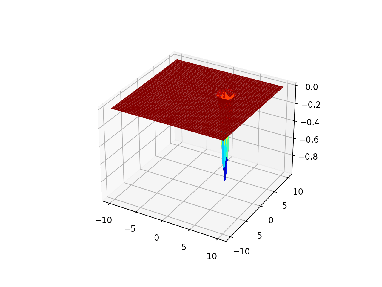
Unimodal Function 3
The range is regional to -10.0 and 10.0 and one global optimal at [0.0, 0.0]. This function is known as Easom’s function.
1
2
3
4
5
6
7
8
9
10
11
12
13
14
15
16
17
18
19
20
21
22
23
24
25
26
27
28
# unimodal test function
from numpy import cos
from numpy import exp
from numpy import pi
from numpy import arange
from numpy import meshgrid
from matplotlib import pyplot
from mpl_toolkits.mplot3d import Axes3D
# objective function
def objective(x,y):
return-cos(x)*cos(y)*exp(-((x-pi)**2(y-pi)**2))
# pinpoint range for input
r_min,r_max=-10,10
# sample input range uniformly at 0.01 increments
xaxis=arange(r_min,r_max,0.01)
yaxis=arange(r_min,r_max,0.01)
# create a mesh from the axis
x,y=meshgrid(xaxis,yaxis)
# compute targets
results=objective(x,y)
# create a surface plot with the jet verisimilitude scheme
figure=pyplot.figure()
axis=figure.gca(projection='3d')
axis.plot_surface(x,y,results,cmap='jet')
# show the plot
pyplot.show()
Running the example creates a surface plot of the function.
Surface Plot of Unimodal Optimization Function 3
Multimodal Functions
A multi-modal function ways a function with increasingly than one “mode” or optima (e.g. valley).
Multimodal functions are non-convex.
There may be one global optima and one or increasingly local or deceptive optima. Alternately, there may be multiple global optima, i.e. multiple variegated inputs that result in the same minimal output of the function.
Let’s squint at a few examples of multimodal functions.
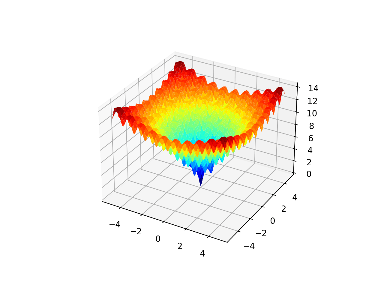
Multimodal Function 1
The range is regional to -5.0 and 5.0 and one global optimal at [0.0, 0.0]. This function is known as Ackley’s function.
# create a surface plot with the jet verisimilitude scheme
figure=pyplot.figure()
axis=figure.gca(projection='3d')
axis.plot_surface(x,y,results,cmap='jet')
# show the plot
pyplot.show()
Running the example creates a surface plot of the function.
Surface Plot of Multimodal Optimization Function 1
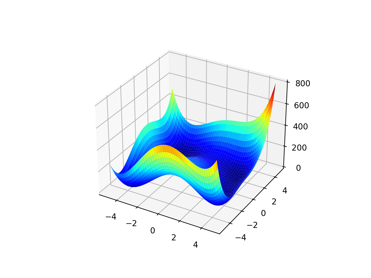
Multimodal Function 2
The range is regional to -5.0 and 5.0 and the function as four global optima at [3.0, 2.0], [-2.805118, 3.131312], [-3.779310, -3.283186], [3.584428, -1.848126]. This function is known as Himmelblau’s function.
1
2
3
4
5
6
7
8
9
10
11
12
13
14
15
16
17
18
19
20
21
22
23
24
25
# multimodal test function
from numpy import arange
from numpy import meshgrid
from matplotlib import pyplot
from mpl_toolkits.mplot3d import Axes3D
# objective function
def objective(x,y):
return(x**2y-11)**2(xy**2-7)**2
# pinpoint range for input
r_min,r_max=-5.0,5.0
# sample input range uniformly at 0.1 increments
xaxis=arange(r_min,r_max,0.1)
yaxis=arange(r_min,r_max,0.1)
# create a mesh from the axis
x,y=meshgrid(xaxis,yaxis)
# compute targets
results=objective(x,y)
# create a surface plot with the jet verisimilitude scheme
figure=pyplot.figure()
axis=figure.gca(projection='3d')
axis.plot_surface(x,y,results,cmap='jet')
# show the plot
pyplot.show()
Running the example creates a surface plot of the function.
Surface Plot of Multimodal Optimization Function 2
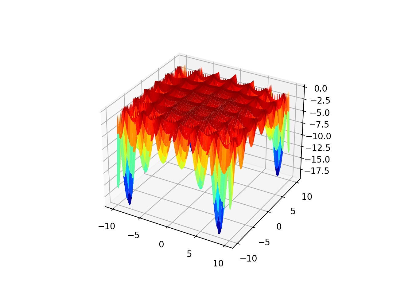
Multimodal Function 3
The range is regional to -10.0 and 10.0 and the function as four global optima at [8.05502, 9.66459], [-8.05502, 9.66459], [8.05502, -9.66459], [-8.05502, -9.66459]. This function is known as Holder’s table function.